library(tidyverse)3 Working with data - Part 2
In this chapter we will continue learning how to manipulate and summarise data using the dplyr package (with a little help from the tidyr package too).
Learning Objectives
At the end of this chapter, learners should be able to:
Apply grouping for more complex analysis of data
Save data frames to a file
Let’s first load the tidyverse
…and read in the MouseZempic® dosage data
# read in the data, like we did in chapter 1
m_dose <- read_delim("data/mousezempic_dosage_data.csv")
Rows: 344 Columns: 9
── Column specification ────────────────────────────────────────────────────────
Delimiter: ","
chr (4): mouse_strain, cage_number, replicate, sex
dbl (5): weight_lost_g, drug_dose_g, tail_length_mm, initial_weight_g, id_num
ℹ Use `spec()` to retrieve the full column specification for this data.
ℹ Specify the column types or set `show_col_types = FALSE` to quiet this message.3.1 Modifying data
So far, we’ve learned how to filter rows and select columns from a data frame. But what if we want to change the data itself? This is where the mutate() function comes in.
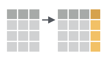
The mutate() function is used to add new columns to a data frame, or modify existing columns, often by performing some sort of calculation. For example, we can add a new column to m_dose that contains the drug dose in mg (rather than g):
m_dose %>%
  # add a new column called drug_dose_mg
  # convert drug_dose_g to mg by multiplying by 1000
  mutate(drug_dose_mg = drug_dose_g * 1000) %>%
  # just select the drug dose columns so we can compare them
  select(drug_dose_g, drug_dose_mg)
# A tibble: 344 × 2
drug_dose_g drug_dose_mg
<dbl> <dbl>
1 0.00181 1.81
2 0.00186 1.86
3 0.00195 1.95
4 NA NA
5 0.00193 1.93
6 0.0019 1.9
7 0.00181 1.81
8 0.00195 1.95
9 0.00193 1.93
10 0.0019 1.9
# ℹ 334 more rowsYou can see that the drug_dose_mg column has been added to the data frame, and it contains, for each row, the value of the drug_dose_g column multiplied by 1000 (NA values are preserved).
These calculations can be as complex as you like, and involve multiple different columns. For example, to add a new column to the m_dose data frame that calculates the weight lost as a percentage of the initial weight:
m_dose %>%
  # calculate the % of initial weight that was lost
  mutate(weight_lost_percent = (weight_lost_g / initial_weight_g) * 100)
# A tibble: 344 × 10
mouse_strain cage_number weight_lost_g replicate sex drug_dose_g
<chr> <chr> <dbl> <chr> <chr> <dbl>
1 CD-1 1A 3.75 rep1 male 0.00181
2 CD-1 1A 3.8 rep1 female 0.00186
3 CD-1 1A 3.25 rep1 female 0.00195
4 CD-1 1A NA rep1 <NA> NA
5 CD-1 1A 3.45 rep1 female 0.00193
6 CD-1 1A 3.65 rep1 male 0.0019
7 CD-1 1A 3.62 rep1 female 0.00181
8 CD-1 1A 4.68 rep1 male 0.00195
9 CD-1 1A 3.48 rep1 <NA> 0.00193
10 CD-1 1A 4.25 rep1 <NA> 0.0019
# ℹ 334 more rows
# ℹ 4 more variables: tail_length_mm <dbl>, initial_weight_g <dbl>,
# id_num <dbl>, weight_lost_percent <dbl>A useful helper function for mutate() is the case_when() function, which allows you to create new columns based on multiple conditions. We do this with the notation case_when(condition1 ~ value1, condition2 ~ value2, ...).
For example, to add a new column to the m_dose data frame that categorises the mice based on how much weight they lost:
m_dose %>%
  # create a new column called weight_loss_category
  mutate(weight_loss_category = case_when(
    weight_lost_g < 4 ~ "Low", # separate conditions with a comma
    weight_lost_g <= 5 ~ "Medium",
    weight_lost_g > 5 ~ "High"
  )) %>%
  select(weight_lost_g, weight_loss_category)
# A tibble: 344 × 2
weight_lost_g weight_loss_category
<dbl> <chr>
1 3.75 Low
2 3.8 Low
3 3.25 Low
4 NA <NA>
5 3.45 Low
6 3.65 Low
7 3.62 Low
8 4.68 Medium
9 3.48 Low
10 4.25 Medium
# ℹ 334 more rowsNote that the conditions are evaluated in order, and the first condition that is TRUE is the one that is used. So if a mouse lost 4.5g, it case_when() would first test if it fits the ‘Low’ category (by checking if 4.5 is less than 4, which it isn’t), and then if it fits the ‘Medium’ category (by checking if 4.5 is less than or equal to 5). Since it is, the mouse would be categorised as ‘Medium’.
Fallback with default value(s)
In the above example, what would happen if a mouse lost -1g (gained weight)? It wouldn’t fit any of the conditions, so it would get an NA in the weight_loss_category column. Sometimes you might want this behaviour, but other times you would prefer to specify a ‘fallback’ category that will be assigned to everything that doesn’t fit in the other categories. You can do this by including a .default = argument at the end of the case_when() function. For example:
m_dose %>%
  # create a new column called weight_loss_category
  mutate(weight_loss_category = case_when(
    weight_lost_g < 4 ~ "Low", # separate conditions with a comma
    weight_lost_g <= 5 ~ "Medium",
    weight_lost_g > 5 ~ "High",
    .default = "Unknown"
  )) %>%
  select(weight_lost_g, weight_loss_category)
# A tibble: 344 × 2
weight_lost_g weight_loss_category
<dbl> <chr>
1 3.75 Low
2 3.8 Low
3 3.25 Low
4 NA Unknown
5 3.45 Low
6 3.65 Low
7 3.62 Low
8 4.68 Medium
9 3.48 Low
10 4.25 Medium
# ℹ 334 more rowsNotice how the NA value in the fourth row is now categorised as ‘Unknown’.
One final thing to note is that mutate() can be used to modify existing columns as well as add new ones. To do this, just use the name of the existing column as the ‘new’ one.
For example, let’s use mutate() together with case_when() to modify the sex column so that it uses M and F instead male and female:
m_dose %>%
  # modify sex column
  mutate(sex = case_when(
    sex == "female" ~ "F",
    sex == "male" ~ "M",
    # if neither, code it as 'X'
    .default = "X"))
# A tibble: 344 × 9
mouse_strain cage_number weight_lost_g replicate sex drug_dose_g
<chr> <chr> <dbl> <chr> <chr> <dbl>
1 CD-1 1A 3.75 rep1 M 0.00181
2 CD-1 1A 3.8 rep1 F 0.00186
3 CD-1 1A 3.25 rep1 F 0.00195
4 CD-1 1A NA rep1 X NA
5 CD-1 1A 3.45 rep1 F 0.00193
6 CD-1 1A 3.65 rep1 M 0.0019
7 CD-1 1A 3.62 rep1 F 0.00181
8 CD-1 1A 4.68 rep1 M 0.00195
9 CD-1 1A 3.48 rep1 X 0.00193
10 CD-1 1A 4.25 rep1 X 0.0019
# ℹ 334 more rows
# ℹ 3 more variables: tail_length_mm <dbl>, initial_weight_g <dbl>,
# id_num <dbl>
Practice exercises
Try these practice questions to test your understanding
1. What line of code would you use to add a new column to the m_dose data frame that converts the tail_length_mm column to cm?
✗m_dose %>% create(tail_length_cm = tail_length_mm / 10)
✗m_dose %>% mutate(tail_length_cm == tail_length_mm / 10)
✔m_dose %>% mutate(tail_length_cm = tail_length_mm / 10)
✗m_dose %>% tail_length_cm = tail_length_mm / 10
2. Explain in words what the following code does:
m_dose %>%
  arrange(desc(weight_lost_g)) %>%
  mutate(weight_lost_rank = row_number())
Hint: the row_number() function returns the number of each row in the data frame (1 being the first row and so on).
✗Adds a new column to the data frame that ranks the mice based on how much weight they lost, with 1 being the mouse that lost the least weight.
✔Adds a new column to the data frame that ranks the mice based on how much weight they lost, with 1 being the mouse that lost the most weight.
✗Adds a new column to the data frame that ranks the mice
✗Does nothing, because the row_number() function has no arguments
3. What is wrong with this R code?
m_dose %>%
  mutate(weight_lost_category = case_when(
    weight_lost_g < 4 ~ "Low"
    weight_lost_g <= 5 ~ "Medium"
    weight_lost_g > 5 ~ "High"
  ))
Error in parse(text = input): <text>:4:5: unexpected symbol
3: weight_lost_g < 4 ~ "Low"
4: weight_lost_g
^ ✗You didn’t include a .default = condition at the end of the case_when() function to act as a fallback
✗You can’t use the case_when() function with the mutate() function
✗weight_lost_g is not a valid column name
✔You need to separate the conditions in the case_when() function with a comma
4. Explain in words what the following code does:
m_dose %>%
  mutate(mouse_strain = case_when(
    mouse_strain == "Black 6" ~ "B6",
    .default = mouse_strain
  ))
Hint: if you’re not sure, try running the code, but pipe it into View() so that you can take a good look at what’s happening in the mouse_strain column.
✗Renames the strains of all the mice to “B6”, regardless of their original strain
✗This code will produce an error
✗Adds a new column that categorises the mice based on their strain, so that any mice from the “Black 6” strain are now called “B6”, and all other strains are left unchanged.
✔Modifies the mouse_strain column so that any mice from the “Black 6” strain are now called “B6”, and all other strains are left unchanged.
Solutions
- The correct line of code to add a new column to the
m_dosedata frame that converts thetail_length_mmcolumn to cm ism_dose %>% mutate(tail_length_cm = tail_length_mm / 10). - The code
m_dose %>% arrange(desc(weight_lost_g)) %>% mutate(weight_lost_rank = row_number())adds a new column to the data frame that ranks the mice based on how much weight they lost, with 1 being the mouse that lost the most weight. First, thearrange(desc(weight_lost_g))function sorts the data frame by theweight_lost_gcolumn in descending order, and then themutate(weight_lost_rank = row_number())function adds a new column that assigns a rank to each row based on its position (row number) in the sorted data frame. - The error is that the conditions in the
case_when()function are not separated by commas. Each condition should be followed by a comma because these are like the arguments in a function. Remeber that it’s optional to include the.default =condition at the end of thecase_when()function. - The code
m_dose %>% mutate(mouse_strain = case_when(mouse_strain == "Black 6" ~ "B6", .default = mouse_strain))modifies themouse_straincolumn so that any mice from the “Black 6” strain are now called “B6”, and all other strains are left unchanged. As we are calling our columnmouse_strain, no new column is being created (we are modifying the existing one) and the.default = mouse_straincondition acts as a fallback to keep the original values (that already exist in themouse_straincolumn) for any rows that don’t match our first condition (strain being “Black 6”).
3.2 Summarising data
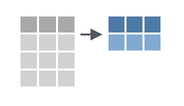
The summarise() (or summarize(), if you prefer US spelling) function is used to calculate summary statistics on your data. It takes similar arguments to mutate(), but instead of adding a new column to the data frame, it returns a new data frame with a single row and one column for each summary statistic you calculate.
For example, to calculate the mean weight lost by the mice in the m_dose data frame:
m_dose %>%
  summarise(mean_weight_lost = mean(weight_lost_g, na.rm = TRUE))
# A tibble: 1 × 1
mean_weight_lost
<dbl>
1 4.20We can also calculate multiple summary statistics at once. For example, to calculate the mean, median, and standard deviation of the weight lost by the mice:
m_dose %>%
  summarise(
    mean_weight_lost = mean(weight_lost_g, na.rm = TRUE),
    median_weight_lost = median(weight_lost_g, na.rm = TRUE),
    sd_weight_lost = sd(weight_lost_g, na.rm = TRUE)
  )
# A tibble: 1 × 3
mean_weight_lost median_weight_lost sd_weight_lost
<dbl> <dbl> <dbl>
1 4.20 4.05 0.802The power of summarising data is really seen when combined with grouping, which we will cover in the next section.
Practice exercises
Try these practice questions to test your understanding
1. Explain in words what the following code does:
m_dose %>%
  summarise(average_tail = mean(tail_length_mm, na.rm = TRUE),
            min_tail = min(tail_length_mm, na.rm = TRUE),
max_tail = max(tail_length_mm, na.rm = TRUE)) ✗Calculates the average, minimum, and maximum tail length of the mice in the m_dose data frame.
✔Produces a data frame containing one column for each of the average, minimum, and maximum tail length of the mice in the m_dose data frame.
✗Finds the average tail length of the mice in the m_dose data frame.
✗Produces a vector containing the average, minimum, and maximum tail length of the mice in the m_dose data frame.
2. What is NOT a valid way to calculate the mean weight lost by the mice in the m_dose data frame?
✗m_dose %>% summarise(mean_weight_lost = mean(weight_lost_g, na.rm = TRUE))
✗m_dose %>% pull(weight_lost_g) %>% mean(na.rm = TRUE)
✗m_dose %>% summarize(mean_weight_lost = mean(weight_lost_g, na.rm = TRUE))
✔m_dose %>% mean(weight_lost_g, na.rm = TRUE)
Solutions
1. The code produces a data frame containing one column for each of the average, minimum, and maximum tail length of the mice in the m_dose data frame.
2. The line of code that is NOT a valid way to calculate the mean weight lost by the mice in the m_dose data frame is m_dose %>% mean(weight_lost_g, na.rm = TRUE). This line of code is incorrect because the mean() function is being used directly on the data frame, rather than within a summarise() function. The other options are valid ways to calculate the mean weight lost by the mice in the m_dose data frame (although note that the second option uses pull() to extract the weight_lost_g column as a vector before calculating the mean, so the mean value is stored in a vector rather than in a data frame).
3.3 Grouping
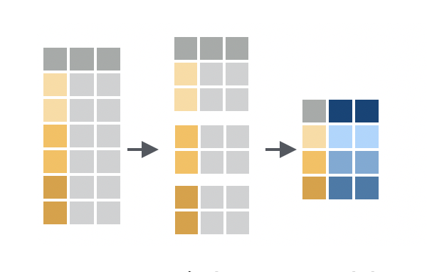
Grouping is a powerful concept in in dplyr that allows you to perform operations on subsets of your data. For example, you might want to calculate the mean weight lost by mice in each cage, or find the mouse with the longest tail in each strain.
We can group data using the .by argument that exists in many dplyr functions, like summarise() and mutate(), and passing it the name(s) of column(s) to group by. For example, to calculate the mean weight lost by mice in each cage:
m_dose %>%
  summarise(
    mean_weight_lost = mean(weight_lost_g, na.rm = TRUE),
    # don't forget it's .by, not by!
    .by = cage_number)
# A tibble: 3 × 2
cage_number mean_weight_lost
<chr> <dbl>
1 1A 3.71
2 3E 4.72
3 2B 3.71Like when we first learned the summarise function above, we give our new column a name (mean_weight_lost), and then we assign its value to be the mean of the weight_lost_g column (with NAs removed). But this time, we also added the .by argument to specify the column we want to group by (cage_number, in this case). This will return a data frame with the mean weight lost by mice in each cage.
Grouping is a powerful tool for exploring your data and can help you identify patterns that might not be obvious when looking at the data as a whole. For example, notice how this grouped summary reveals that mice in cage 3E lost more weight than those in the other two cages.
It’s also possible to group by multiple columns by passing a vector of column names to the .by argument. For example, to calculate the mean weight lost by mice in each cage and strain:
m_dose %>%
  summarise(mean_weight_lost = mean(weight_lost_g, na.rm = TRUE),
  # group by both cage_number and mouse_strain
    .by = c(cage_number, mouse_strain))
# A tibble: 5 × 3
cage_number mouse_strain mean_weight_lost
<chr> <chr> <dbl>
1 1A CD-1 3.71
2 3E CD-1 3.71
3 2B CD-1 3.69
4 3E Black 6 5.08
5 2B BALB C 3.73Of course, mean() is not the only function that we can use within summarise(). We can use any function that takes a vector of values and returns a single value, like median(), sd(), or max(). We can also use multiple functions at once, by giving each column a name and specifying the function we want to use. In the following code we first drop NA values from the weight_lost_g column, to avoid repeating na.rm = TRUE:
m_dose %>%
  drop_na(weight_lost_g) %>%
  summarise(
    n = n(),
    mean_weight_lost = mean(weight_lost_g),
    median_weight_lost = median(weight_lost_g),
    sd_weight_lost = sd(weight_lost_g),
    max_weight_lost = max(weight_lost_g),
    min_weight_lost = min(weight_lost_g),
    .by = cage_number)
# A tibble: 3 × 7
cage_number n mean_weight_lost median_weight_lost sd_weight_lost
<chr> <int> <dbl> <dbl> <dbl>
1 1A 51 3.71 3.7 0.445
2 3E 167 4.72 4.78 0.783
3 2B 124 3.71 3.69 0.417
# ℹ 2 more variables: max_weight_lost <dbl>, min_weight_lost <dbl>Here, we also used the n() function to calculate the number of mice in each cage. This is a special helper function that works within summarise to count the number of rows in each group.
To
.by or not to .by?
In the dplyr package, there are two ways to group data: using the .by argument within various functions (as we have covered so far), or using the group_by() function, then performing your operations and ungrouping with ungroup().
For example, we’ve seen above how to calculate the mean weight lost by mice in each cage using the .by argument:
m_dose %>%
  summarise(mean_weight_lost = mean(weight_lost_g, na.rm = TRUE), .by = cage_number)
# A tibble: 3 × 2
cage_number mean_weight_lost
<chr> <dbl>
1 1A 3.71
2 3E 4.72
3 2B 3.71But we can also do the same using group_by() and ungroup():
m_dose %>%
  group_by(cage_number) %>%
  summarise(mean_weight_lost = mean(weight_lost_g, na.rm = TRUE)) %>%
  ungroup()
# A tibble: 3 × 2
cage_number mean_weight_lost
<chr> <dbl>
1 1A 3.71
2 2B 3.71
3 3E 4.72The two methods are equivalent, but using the .by argument within functions can be more concise and easier to read. Still, it’s good to be aware of group_by() and ungroup() as they are widely used, particularly in older code.
Although grouping is most often used with summarise(), it can be used with dplyr functions too. For example mutate() function can also be used with grouping to add new columns to the data frame based on group-specific calculations. Let’s say we wanted to calculate the Z-score (also known as the standard score) to standardise the weight lost by each mouse within each strain.
As a reminder, the formula for calculating the Z-score is \(\frac{x - \mu}{\sigma}\), where \(x\) is the value (in our case the weight_lost_g column), \(\mu\) is the mean, and \(\sigma\) is the standard deviation.
We can calculate this for each mouse in each strain using the following code:
m_dose %>%
  # remove NAs before calculating the mean and SD
  filter(!is.na(weight_lost_g)) %>%
  mutate(weight_lost_z = (weight_lost_g - mean(weight_lost_g)) / sd(weight_lost_g), .by = mouse_strain) %>%
  # select the relevant columns
  select(mouse_strain, weight_lost_g, weight_lost_z)
# A tibble: 342 × 3
mouse_strain weight_lost_g weight_lost_z
<chr> <dbl> <dbl>
1 CD-1 3.75 0.108
2 CD-1 3.8 0.217
3 CD-1 3.25 -0.983
4 CD-1 3.45 -0.547
5 CD-1 3.65 -0.110
6 CD-1 3.62 -0.165
7 CD-1 4.68 2.12
8 CD-1 3.48 -0.492
9 CD-1 4.25 1.20
10 CD-1 3.3 -0.874
# ℹ 332 more rowsUnlike when we used .by with summarise(), we still get the same number of rows as the original data frame, but now we have a new column weight_lost_z that contains the Z-score for each mouse within each strain. This could be useful for identifying outliers or comparing the weight lost by each mouse to the average for its strain.
Practice exercises
Try these practice questions to test your understanding
1. Which line of code would you use to calculate the median tail length of mice belonging to each strain in the m_dose data frame?
✗m_dose %>% summarise(median_tail_length = median(tail_length_mm), .by = mouse_strain)
✔m_dose %>% summarise(median_tail_length = median(tail_length_mm, na.rm = TRUE), .by = mouse_strain)
✗m_dose %>% summarise(median_tail_length = median(tail_length_mm, na.rm = TRUE), by = mouse_strain)
✗m_dose %>% mutate(median_tail_length = median(tail_length_mm, na.rm = TRUE), .by = mouse_strain)
2. Explain in words what the following code does:
m_dose %>%
summarise(max_tail_len = max(tail_length_mm, na.rm = TRUE), .by = c(mouse_strain, replicate)) ✗Calculates the maximum tail length of all mice for each strain in the m_dose data frame
✗Calculates the maximum tail length of all mice for each replicate in the m_dose data frame
✗Calculates the maximum tail length of all mice in the m_dose data frame
✔Calculates the maximum tail length of mice in each unique combination of strain and replicate in the m_dose data frame.
3. I want to count how many male and how many female mice there are for each strain in the m_dose data frame. Which line of code would I use?
✗m_dose %>% summarise(count = n(), .by = sex)
✗m_dose %>% summarise(count = n(), .by = mouse_strain)
✔m_dose %>% summarise(count = n(), .by = c(mouse_strain, sex))
✗m_dose %>% summarise(count = n(), .by = mouse_strain, sex)
4. I want to find the proportion of weight lost by each mouse in each cage in the m_dose data frame. Which line of code would I use?
✗m_dose %>% summarise(weight_lost_proportion = weight_lost_g / sum(weight_lost_g, na.rm = TRUE), .by = cage_number)
✔m_dose %>% mutate(weight_lost_proportion = weight_lost_g / sum(weight_lost_g, na.rm = TRUE), .by = cage_number)
✗m_dose %>% mutate(weight_lost_proportion = weight_lost_g / sum(weight_lost_g, na.rm = TRUE, .by = cage_number))
✗m_dose %>% mutate(weight_lost_proportion = weight_lost_g / sum(weight_lost_g, na.rm = TRUE))
Solutions
- The correct line of code to calculate the median tail length of mice belonging to each strain in the
m_dosedata frame ism_dose %>% summarise(median_tail_length = median(tail_length_mm, na.rm = TRUE), .by = mouse_strain). Remember to usena.rm = TRUEto remove any missing values before calculating the median, and to use.byto specify the column to group by (notby). Seeing as we want to calculate the median (collapse down to a single value per group), we need to usesummarise()rather thanmutate(). - The code
m_dose %>% summarise(max_tail_len = max(tail_length_mm, na.rm = TRUE), .by = c(mouse_strain, replicate))calculates the maximum tail length of mice in each unique combination of strain and replicate in them_dosedata frame. - The correct line of code to count how many male and how many female mice there are for each strain in the
m_dosedata frame ism_dose %>% summarise(count = n(), .by = c(mouse_strain, sex)). We need to group by bothmouse_strainandsexto get the count for each unique combination of strain and sex. Don’t forget that we specify the column names as a vector when grouping by multiple columns. - The correct line of code to find the proportion of weight lost by each mouse in each cage in the
m_dosedata frame ism_dose %>% mutate(weight_lost_proportion = weight_lost_g / sum(weight_lost_g, na.rm = TRUE), .by = cage_number). We usemutate()because we want a value for each mouse (each row in our data), rather than to collapse down to a single value for each group (cage number in this case). Be careful that you use the.byargument within themutate()function call, not within thesum()function by mistake (this is what is wrong with the third option).
3.4 Saving data to a file
Once you’ve cleaned and transformed your data, you’ll often want to save it to a file so that you can use it in other programs or share it with others. The write_csv() and write_tsv() functions from the readr package are a great way to do this. They take two arguments - the data frame you want to save and the file path where you want to save it.
For example, let’s say I want to save my summary table of the weight lost by mice in each cage to a CSV file called cage_summary_table.csv:
# create the summary table
# and assign it to a variable
cage_summary_table <- m_dose %>%
  summarise(
    n = n(),
    mean_weight_lost = mean(weight_lost_g, na.rm = TRUE),
    median_weight_lost = median(weight_lost_g, na.rm = TRUE),
    sd_weight_lost = sd(weight_lost_g, na.rm = TRUE),
    .by = cage_number)

# save the data to a CSV file
write_csv(cage_summary_table, "cage_summary_table.csv")
CSV files are particularly great because they can be easily read into other software, like Excel.
It’s also possible to use the write_*() functions along with a pipe:
m_dose %>%
  drop_na(weight_lost_g) %>%
  summarise(
    n = n(),
    mean_weight_lost = mean(weight_lost_g),
    median_weight_lost = median(weight_lost_g),
    sd_weight_lost = sd(weight_lost_g),
    .by = cage_number) %>%
  write_csv("cage_summary_table.csv")
Remember here that the first argument (the data frame to save) is passed on by the pipe, so the only argument in the brackets is the second one: the file path.
3.5 Summary
Here’s what we’ve covered in this chapter:
The basic dplyr verbs
mutate(), andarrange()and how they can be used to tidy and analyse data.The
summarise()function and how it can be used to calculate summary statistics on your data, as well as the power of grouping data with the.byargument.
Why does data need to be tidy anyway?
In this chapter, we’ve been focusing on making our data ‘tidy’: that is, structured in a consistent way that makes it easy to work with. A nice visual illustration of tidy data and its importance can be found here.
3.5.1 Practice questions
What would be the result of evaluating the following expressions? You don’t need to know these off the top of your head, use R to help! (Hint: some expressions might give an error. Try to think about why)
m_dose %>% mutate(weight_lost_kg = weight_lost_g / 1000)m_dose %>% summarise(mean_weight_lost = mean(weight_lost_g, na.rm = TRUE))m_dose %>% summarise(mean_weight_lost = mean(weight_lost_g, na.rm = TRUE), .by = cage_number)
I want to add a new column to the
m_dosedata frame that converts themouse_straincolumn to lowercase. Hint: you can use thetolower()function in R to convert characters to lowercase. Look up its help page by typing?tolowerin the R console to see how to use it.How could you find the maximum tail length for each unique combination of sex and mouse strain in the
m_dosedata frame?Write a line of code to save the result of Q5 to a CSV file called
max_tail_length.csv.
Solutions
- The result of evaluating the expressions would be:
- A data frame with an additional column
weight_lost_kgthat contains the weight lost in kilograms. - A data frame with the mean weight lost by all mice.
- A data frame with the mean weight lost by mice in each cage.
- A data frame with an additional column
- To add a new column to the
m_dosedata frame that converts themouse_straincolumn to lowercase, you can usemutate()as follows`:
m_dose %>%
  mutate(mouse_strain_lower = tolower(mouse_strain))
# A tibble: 344 × 10
mouse_strain cage_number weight_lost_g replicate sex drug_dose_g
<chr> <chr> <dbl> <chr> <chr> <dbl>
1 CD-1 1A 3.75 rep1 male 0.00181
2 CD-1 1A 3.8 rep1 female 0.00186
3 CD-1 1A 3.25 rep1 female 0.00195
4 CD-1 1A NA rep1 <NA> NA
5 CD-1 1A 3.45 rep1 female 0.00193
6 CD-1 1A 3.65 rep1 male 0.0019
7 CD-1 1A 3.62 rep1 female 0.00181
8 CD-1 1A 4.68 rep1 male 0.00195
9 CD-1 1A 3.48 rep1 <NA> 0.00193
10 CD-1 1A 4.25 rep1 <NA> 0.0019
# ℹ 334 more rows
# ℹ 4 more variables: tail_length_mm <dbl>, initial_weight_g <dbl>,
# id_num <dbl>, mouse_strain_lower <chr>- You can use the
max()function withinsummarise(.by = c(sex, mouse_strain))to find the maximum tail length of each unique sex/mouse strain combination:
m_dose %>%
  summarise(max_tail_length = max(tail_length_mm, na.rm = TRUE), .by = c(sex, mouse_strain))
# A tibble: 8 × 3
sex mouse_strain max_tail_length
<chr> <chr> <dbl>
1 male CD-1 21.5
2 female CD-1 20.7
3 <NA> CD-1 20.2
4 female Black 6 15.5
5 male Black 6 17.3
6 <NA> Black 6 15.7
7 female BALB C 19.4
8 male BALB C 20.8- To save the result of Q5 to a CSV file called
max_tail_length.csv, you can use thewrite_csv()function, either by using a pipe to connect it to the code you wrote previously:
m_dose %>%
  summarise(max_tail_length = max(tail_length_mm, na.rm = TRUE), .by = c(sex, mouse_strain)) %>%
  write_csv("max_tail_length.csv")
Or by assigning this result to a variable and then saving it to a file:
max_tail_length <- m_dose %>%
  summarise(max_tail_length = max(tail_length_mm, na.rm = TRUE), .by = c(sex, mouse_strain))

write_csv(max_tail_length, "max_tail_length.csv")