In this chapter we will combine all the skills we have learned so far to perform a complete analysis of a small dataset.
Learning Objectives
At the end of this chapter, learners should be able to:
Describe the key steps in data analysis (exploration, manipulating and plotting)
Understand how pivot and join functions can be used to reshape and combine entire data frames
5.1 Introduction to the dataset
In this chapter we will use the mousezempic dosage data m_dose and mouse expression data m_exp data frames, which contain information about the mice including mousezempic dose, and their gene expression levels, respectively.
library(tidyverse)library(patchwork)# read in dosage datam_dose <-read_csv("data/mousezempic_dosage_data.csv")m_dose
We have used read_csv() for the mouse data and read_tsv() for the expression data. These are for reading data separated by commas and tab characters respectively. The readr package also provides read_delim() to let the package guess your delimiter, but if you know the format of your file then it’s good practice to use the appropriate reading function for more predictable behaviour.
Caution
There’s nothing stopping someone from naming a file file.csv while having tab-separated data inside. This happens quite often in real-world data so it’s a good idea to have a quick look at the data in an text editor before reading it in.
5.2 Tidy Data
The tidyverse revolves around an important concept called “tidy data”. This is a specific representation of tabular data that is considered easy to work with. Tidy data is roughly defined as tabular data that contains:
Individual variables in columns
Individual observations in rows
One data value in each cell
Having individual variables in columns makes then accessible for performing tidyverse operations like select(), mutate(), filter() and arrange(). If variables were not stored as columns, then these functions would not be able to access them by name.
Having individual observations in rows is important because it associates all variables of each observation with the same row. If the data from one observation is spread across multiple rows then it is easy to incorrect summaries from the summarise() function. When using the filter() function with tidy data, you can expect to keep all the data for an observation or none at all. When the data for observations is split over different rows, it’s possible to unknowingly lose partial data from observations.
Having a single value in each cell makes it possible to perform meaningful computations for the values, for example you cannot take a mean() of a column of values that contain multiple different values.
Although tidy data is the easiest to work with, it’s often necessary to alter the format of your data for plotting or table displays. It’s a good idea to keep your core data in a tidy format and treating plot or table outputs as representations of that tidy data.
Note
Most data you encounter will not be tidy, the first part of data analysis is usually called “data-wranging” and involves tidying up your data so it is easier to use for downstream analysis.
5.3 Reshaping and combining data
The filter(), select(), mutate() and summarise() functions we learned last chapter all operate along either the columns or the rows of data. Combining these operations cleverly can answer the majority of questions about your data. However, there are two useful families of functions: pivot for reshaping your data and join for combining your data from shared columns.
5.3.1 Reshaping data with pivot functions
Pivoting is a way to change the shape of your tibble.
Pivoting longer reshapes the data to transfer data stored in columns into rows, resulting in more rows and fewer columns.
Pivoting wider is the reverse, moving data from rows into columns.
Pivot functions allow you to change the structure of your data frame
The pivot_longer() function is used to pivot data from wide to long format, and the pivot_wider() function is used to pivot data from long to wide format.
5.3.1.1 Pivot wider
A common use case for pivot_wider() is to make a contingency table, which shows the number of observations for each combination of two variables. This is often easier to read than the same information in long format.
For example, let’s say we want to create a table that shows how many mice there are of each strain, in each cage number. We can achieve this in a long format using summarise() as we learned in the previous section:
# A tibble: 5 × 3
  cage_number mouse_strain n_mice
  <chr>       <chr>         <int>
1 1A          CD-1             52
2 3E          CD-1             44
3 2B          CD-1             56
4 3E          Black 6         124
5 2B          BALB C           68
For the specific task of counting, we can achieve the same effect using the count() tidyverse function.
m_dose %>%count(cage_number, mouse_strain, name ="n_mice")
# A tibble: 5 × 3
  cage_number mouse_strain n_mice
  <chr>       <chr>         <int>
1 1A          CD-1             52
2 2B          BALB C           68
3 2B          CD-1             56
4 3E          Black 6         124
5 3E          CD-1             44
This summarises by each combination of cage_number and mouse_strain, with the n() function giving the count of data belonging to that combination.
To get a contingency table, we wish to have the information in the mouse_strain column displayed along the column names and the values of n_mice becoming the values of the cells in the new table. Since the goal is to make the table wider, we use the pivot_wider() function. To achieve this, we instruct the pivot_wider() function to take names from the mouse_strain column and the values from the n_mice column.
# A tibble: 3 × 4
  cage_number `CD-1` `BALB C` `Black 6`
  <chr>        <int>    <int>     <int>
1 1A              52       NA        NA
2 2B              56       68        NA
3 3E              44       NA       124
This has transformed our data into a contingency table, with NA where no data corresponding data exists for the specific cage_number and mouse_strain combination.
We can do the same thing to see how many of each mouse strains is in each of our experiment replicates.
Data can often arrive in the form similar to the contingency table we constructed. Although this data is easy to read, it is difficult to operate on using tidyverse functions because the mouse_strain data is now stored in the column names and not inside a column we can use as a variable. In order to make this kind of data tidy, we use the pivot_longer() function, which will create a pair of columns from the column names and the value of the corresponding cell.
To demonstrate pivot_longer(), we will use the m_exp that we downloaded earlier. This data frame contains the expression levels of two genes (TH and PRLH) suspected to be upregulated in mice taking MouseZempic, as well as one housekeeping gene (HPRT1), all measured in triplicate.
The data is currently in wide format, with each row representing a different mouse (identified by its id_num) and each column representing a different measurement of a gene. To reshape this data into a long format (where each measurement is contained on a separate row), we can use pivot_longer(), specifying three arguments:
cols: the columns to pivot from. You can use selection helpers like contains() or starts_with() to easily select multiple columns at once.
names_to: the name of a new column that will contain the original column names.
values_to: the name of a new column that will contain the values from the original columns.
In this particular case here’s what the code would look like:
Pivoting can be a bit tricky to get your head around! Often when you’re doing analysis, you’ll run into the problem of knowing that you need to pivot, but not knowing exactly what arguments to use. In these cases, it can be helpful to look at examples online, like those in the R for Data Science book.
5.3.2 Separating data in a column
When we look at the measurement column we see that it contains two pieces of information. The gene being measured and the replicate number separated by “_”. We can use the separate() function to split this data into individual columns so that one column does not contain multiple variables.
m_exp_separate <- m_exp_long %>%separate(measurement, into =c("gene", "replicate"), sep ="_")m_exp_separate
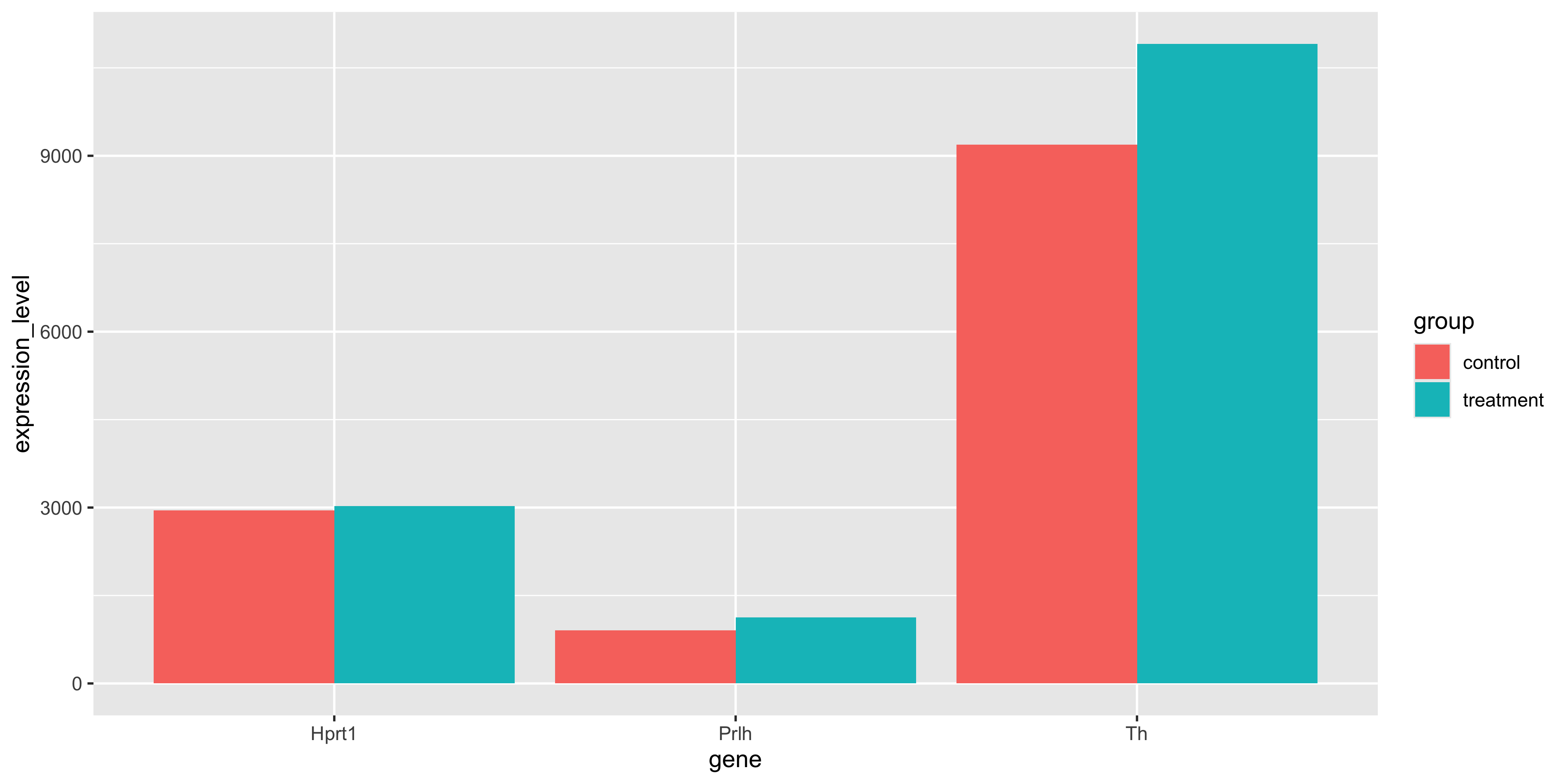
We may also want to get the average expression level of each gene within each experimental group and plot it as a bar chart.
m_exp_rep_summed %>%summarise(expression_level =mean(expression_level),.by =c(group, gene) ) %>%ggplot(aes(x = gene, y = expression_level, fill = group)) +geom_col(position ="dodge")
We see that all 3 genes are slightly higher in the treatment group.
5.3.4 Reshaping for plotting
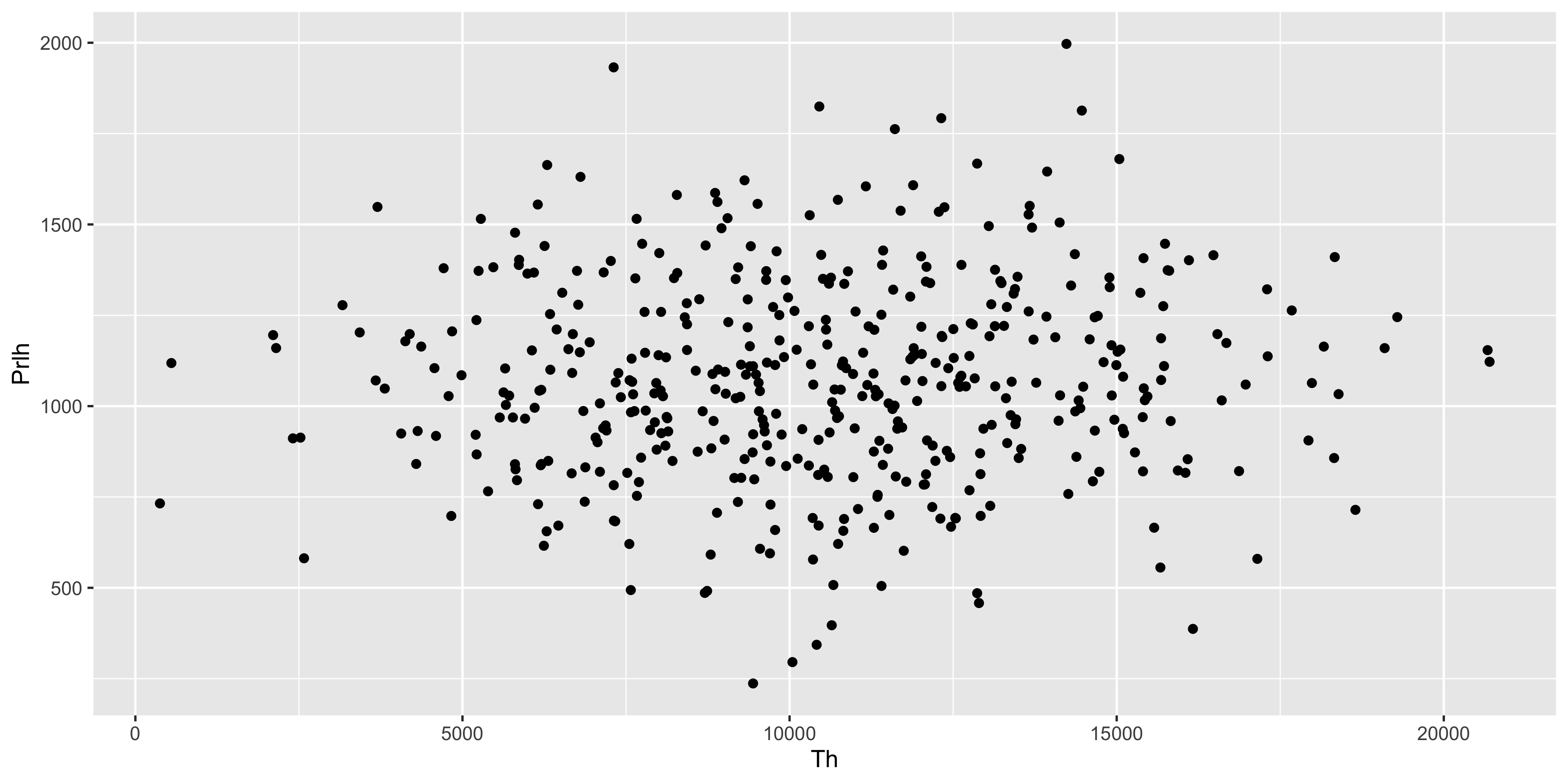
Suppose we wanted to plot the value of two genes against each other. We would need the expression values of genes to be in individual columns. However we have lost this structure after using pivot_longer(). We can restore it using pivot_wider() after we have summarised the replicates.
With the replicate aggregated expression levels in individual columns, we can now plot the gene expression values against each other.
m_exp_rep_summed_wide %>%ggplot( aes(x = Th, y = Prlh)) +geom_point()
Practice exercise
Make all the pair-wise scatter plots and assemble them together using patchwork. There should be plots of:
Th vs Prlh
Th vs Hprt1
Prlh vs Hprt1
5.3.5 Combining data with join functions
Data analysis typically involves multiple tables of data. Often there will be tables that are contain related information that must be combined to answer the questions you’re interested in. Tables that are related to each other tend to have one or more columns in common, and are referred to as “relational data”. Combining relational data in useful ways requires the join family of functions. In general joins can accomplish two tasks
Add new variables to an existing table containing additional information.
Filter observations in one table based on whether or not they match observations in another table.
Both of the above at the same time.
The left_join() function allows you to combine two data frames
A common and basic join is the left_join(). It takes two data frame as arguments and optionally a vector of common columns to perform the join on. The reason it’s called a left-join because it retains all rows from the left data frame while adding on columns from the right data frame only when the data in the designed joining column(s) match.
For example, we can join the m_dose data frame with the m_exp_rep_summed_wide data frame based on the id_num column, which is common to both data frames:
left_join(m_dose, m_exp_rep_summed_wide, by ="id_num")
The m_dose contains information about characteristics of each mouse, while the m_exp_rep_summed_wide contains the replicate-summed gene expressions of the mice. Each data frame has an id_num column that relates the data from the two data frames together, and we have joined them into one table that contains both the data about the mice as well as the expression of their genes.
With the left_join(), if there is a id_num value that exists in the right data frame but not found in the left, then that data will not be present in the joined table. For any id_num that appears only in the left but not the right data frame, the values in the newly created columns will be NA.
Caution
If the values from the left data frame matches to multiple rows of the column in the right data frame, the left_join() will duplicate the data from the left data frame for each match to the right. This can cause issues with downstream summarisation if not carefully considered.
5.3.5.1 Joining with mismatched column names
Often the column containing the matching information has different names in different data frames. For example what might be called “id_num” in one data frame could also be called “mouse_id” in another data frame. In those cases the by argument of left_join() can be formatted to let the function know which column in the left data frame matches to which column on the right.
We will demonstrate this by renaming the id_num column in the m_dose to mouse_id and using it to perform the join instead. We will use the join_by(mouse_id == id_num) helper function for the by argument to specify the different columns we wish to join by.
# rename id_num to mouse_idm_dose_data_new <- m_dose %>%rename(mouse_id = id_num)m_dose_data_new
# perform left join by matching mouse_id of the left data frame to id_num of the right data framem_joined_data <-left_join( m_dose_data_new, m_exp_rep_summed_wide,by =join_by(mouse_id == id_num)) %>%drop_na() # keep only rows without NAm_joined_data
When joining data frames with mismatched column names, the column name from the left data frame argument will be retained for the joined result.
Note
An older syntax exists for the by argument that would look like by = c("mouse_id" = "id_num"). This does the same thing as what is shown above but the documentation now recommends the new syntax which allows for flexible options like joining to the closest.
5.4 Visualising & testing expression between strains
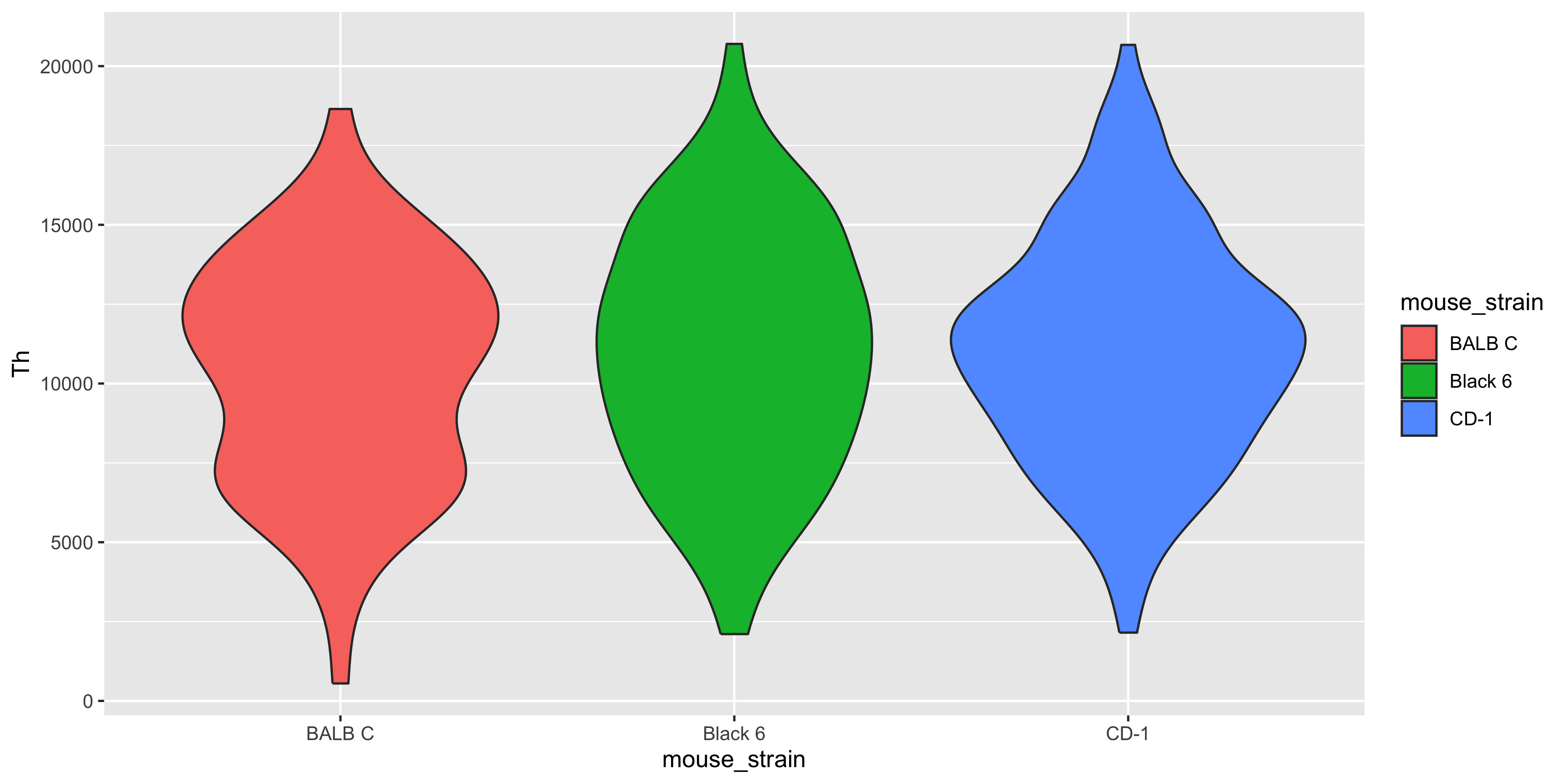
With the joined data we now have more information about the mice in addition to the expression data. So we can check if there is any significant difference in gene expressions between mouse strains.
m_joined_data %>%ggplot( aes(x = mouse_strain, y = Th, fill = mouse_strain)) +geom_violin()
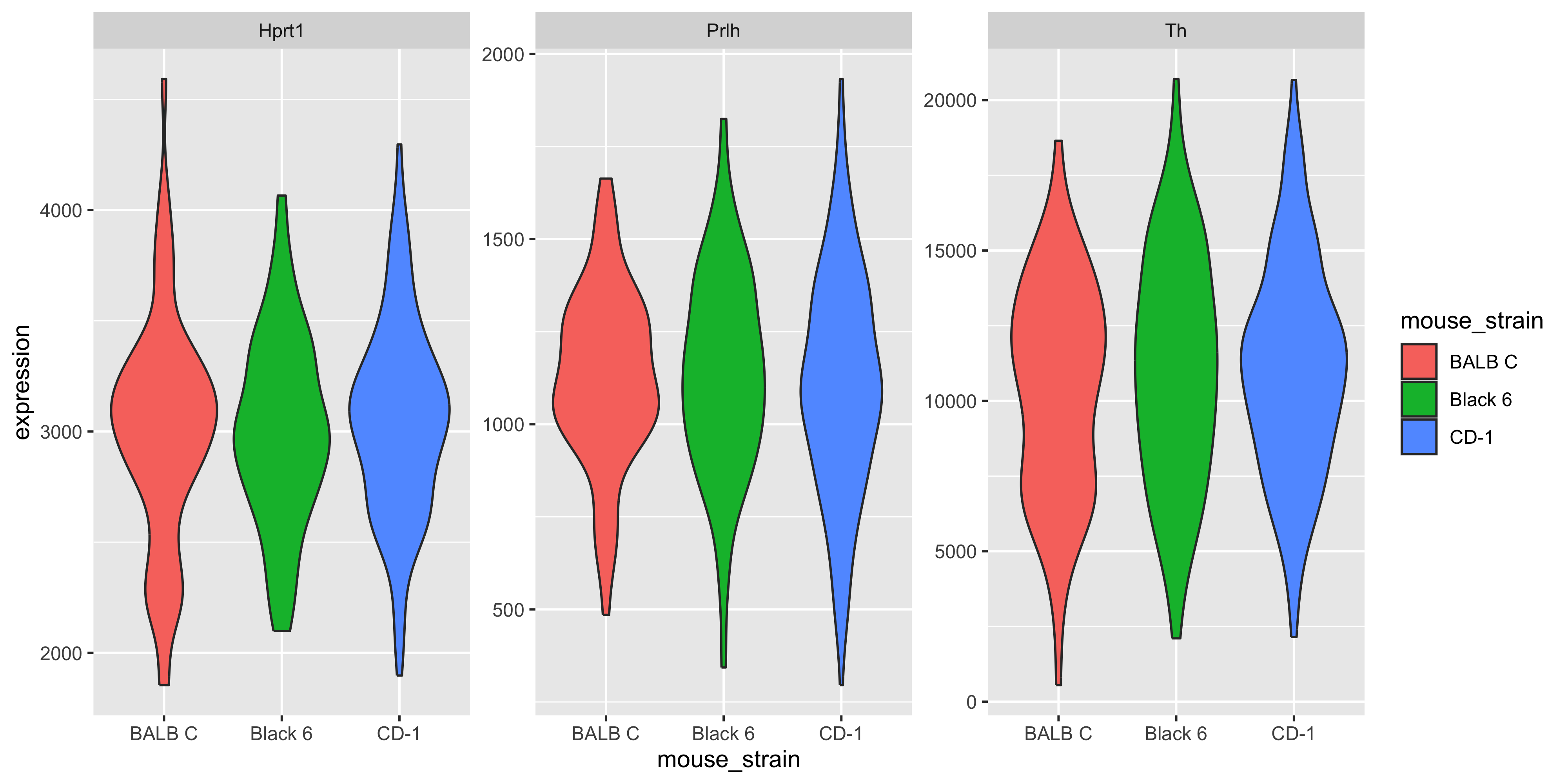
If we wanted to plot all 3 genes, one way is to make 3 different plots, but we can also use facets. However to use facets we would need to have the faceting variable in a column, and currently our gene names are in the column names. So we must use pivot_longer().
Now that the gene variable is in a column, we can use this information to create our faceted plot. We use facet_wrap() with the scales = "free_y" argument so each gene can have its own y-axis.
m_joined_data_long %>%ggplot( aes(x = mouse_strain, y = expression, fill = mouse_strain)) +geom_violin() +facet_wrap(~gene, scales ="free_y")
There doesn’t appear to be clear differences in the expression of these three genes between the haplotypes.
5.4.1 Simple linear model (discrete x)
To fit a line through the gene expression values of each mouse genotype, and test for significance of the x~y relationship, we can use a handy function lm_test() from the tidyrstats library.
library(tidyrstats)
This function takes a long-format data frame as input, and the formula for the linear model we want to fit. (We will read more about linear models in later chapters). For this test, for each gene, we want to know whether the response (gene expression ; aka ‘y’), changes significantly with the predictor (mouse strain ; aka ‘x’). The model formula will be y ~ x1, that is expression ~ mouse_strain.
Our intuition from the violin plots is correct. None of the genes show significant differences in expression between the Black6 vs the reference (BALBC), nor the CD-1 vs the reference. Note that all of the P values are > 0.05, meaning we dont have enough evidence to reject the null hypothesis.
5.5 Visualising & testing relationships between dosage and genes
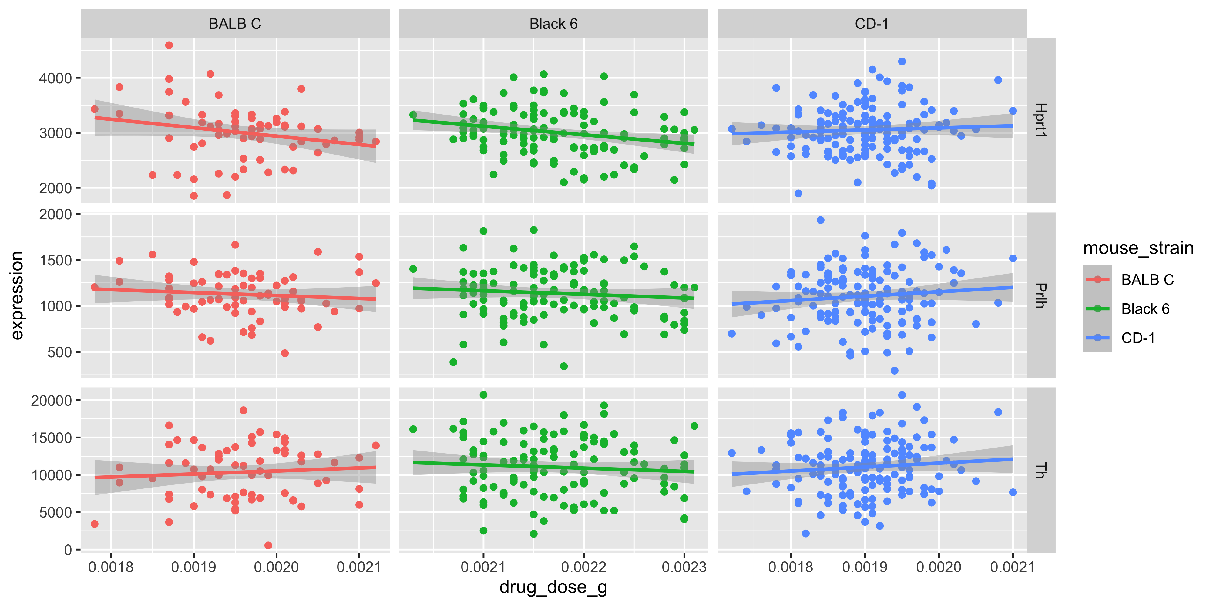
With the joined data frame we can also visualise the relationship between the drug dosage and the genes, separated by mouse strain. We do this by using our m_joined_data_long to plot with facet_grid() specifying the layout of our grid.
m_joined_data_long %>%ggplot(aes(x = drug_dose_g, y = expression, color = mouse_strain)) +geom_point() +geom_smooth(method ="lm") +facet_grid(cols =vars(mouse_strain), rows =vars(gene), scales ="free")
`geom_smooth()` using formula = 'y ~ x'
Although very minor, there appears to be some effect of dosage on gene expression that is strain specific.
5.5.1 Simple linear model (continuous x)
Again, we can test this using lm_test(), where y is expression, and x is now the continuous variable drug_dose_g. We are testing the association for each gene in each mouse strain, by grouping the input data before lm_test(). Note this is different from correcting for gene and mouse strain as covariates, because the model only tests one gene-strain combination at a time.
Here we can see, in fact there is a significant association between Mousezempic drug dose and gene expression: within the Black 6 strain, for the Hprt1 gene.
Stating statistical findings
From our summary table above, can you finish this sentence which is the formal statement of results from a linear model?
“In the Black 6 mouse strain, for every 1 gram increase in drug dose, on average, Hprt1 gene expression …”
We can save our newly transformed and joined data frames for easy access using the save() command, which takes any number of environment objects, and a new Rdata format file name as arguments:
We can look at another dataset containing tuberculosis (TB) cases broken down by year, country, age, gender, and diagnosis method. The data comes from the 2014 World Health Organization Global Tuberculosis Report and is typical of many real-life datasets in terms of structure. There are redundant columns, odd variable codes and missing values.
We want to tidy it up using the tools we have learned in order to try to extract some information from this data.
who
# A tibble: 7,240 × 60
   country  iso2  iso3   year new_sp_m014 new_sp_m1524 new_sp_m2534 new_sp_m3544
   <chr>    <chr> <chr> <dbl>       <dbl>        <dbl>        <dbl>        <dbl>
 1 Afghani… AF    AFG    1980          NA           NA           NA           NA
 2 Afghani… AF    AFG    1981          NA           NA           NA           NA
 3 Afghani… AF    AFG    1982          NA           NA           NA           NA
 4 Afghani… AF    AFG    1983          NA           NA           NA           NA
 5 Afghani… AF    AFG    1984          NA           NA           NA           NA
 6 Afghani… AF    AFG    1985          NA           NA           NA           NA
 7 Afghani… AF    AFG    1986          NA           NA           NA           NA
 8 Afghani… AF    AFG    1987          NA           NA           NA           NA
 9 Afghani… AF    AFG    1988          NA           NA           NA           NA
10 Afghani… AF    AFG    1989          NA           NA           NA           NA
# ℹ 7,230 more rows
# ℹ 52 more variables: new_sp_m4554 <dbl>, new_sp_m5564 <dbl>,
#   new_sp_m65 <dbl>, new_sp_f014 <dbl>, new_sp_f1524 <dbl>,
#   new_sp_f2534 <dbl>, new_sp_f3544 <dbl>, new_sp_f4554 <dbl>,
#   new_sp_f5564 <dbl>, new_sp_f65 <dbl>, new_sn_m014 <dbl>,
#   new_sn_m1524 <dbl>, new_sn_m2534 <dbl>, new_sn_m3544 <dbl>,
#   new_sn_m4554 <dbl>, new_sn_m5564 <dbl>, new_sn_m65 <dbl>, …
The first thing we notice is that country, iso2 and iso3 all seem to be different encodings for the country. The year column is fine as a variable but the rest of the columns seem appear to be coding values in the column names. There are numeric values in the cells, and since we know this dataset is supposed to contain case numbers, and no column clearly denotes this, we suspect that the values in the columns are case numbers with the column names being descriptive of the cases.
Since we believe that many of these column names are in fact encoding data, we want to pivot_longer() to put that information in a column for further processing.
# pivot longer with columns 5 to 60, drop NA valueswho_long <- who %>%pivot_longer(cols =5:60, # alternatively contains("_")names_to ="description",values_to ="cases",values_drop_na =TRUE )who_long
# A tibble: 76,046 × 6
   country     iso2  iso3   year description  cases
   <chr>       <chr> <chr> <dbl> <chr>        <dbl>
 1 Afghanistan AF    AFG    1997 new_sp_m014      0
 2 Afghanistan AF    AFG    1997 new_sp_m1524    10
 3 Afghanistan AF    AFG    1997 new_sp_m2534     6
 4 Afghanistan AF    AFG    1997 new_sp_m3544     3
 5 Afghanistan AF    AFG    1997 new_sp_m4554     5
 6 Afghanistan AF    AFG    1997 new_sp_m5564     2
 7 Afghanistan AF    AFG    1997 new_sp_m65       0
 8 Afghanistan AF    AFG    1997 new_sp_f014      5
 9 Afghanistan AF    AFG    1997 new_sp_f1524    38
10 Afghanistan AF    AFG    1997 new_sp_f2534    36
# ℹ 76,036 more rows
It doesn’t look like the values in description are unique, so we can try to count them to get a sense of what we’re dealing with. It will show us the unique values as well as the counts for each value.
Some patterns emerge, and it maybe be possible to guess at exactly what these values mean. For example we see the presence of “m” and “f” in the encoding which probably encodes sex. Luckily we have a data dictionary ready from the source that tells us what this means.
The first part tells us if the data is new or old, in this case all data is new.
The next part describe the type of TB:
rel for relapse
ep for extrapulmonary
sn for pulmonary TB that cannot be diagnosed with a pulmonary smear (smear negative)
sp for pulmonary TB that can be diagnosed with a smear (smear positive)
The sex of the patient. Males and females denoted by m and f respectively.
The 7 age groups the data is divided into:
014: 0 - 14 years old
1524: 15 - 24 years old
2534: 25 - 34 years old
3544: 35 - 44 years old
4554: 45 - 54 years old
5564: 55 - 64 years old
65: 65 or older
5.7.1 String manupulation
Armed with that knowledge we can begin to tidy up our dataset! The first thing we will do is tidy up the description column, we will do this with some string manipulation functions from the tidyverse. These functions help us manipulate strings programatically and are essential in dealing with real-world data.
Some useful functions for string manipulation include:
str_replace(string, pattern, replacement): replaces the pattern in the string with the replacement.
str_extract(string, pattern): extracts the part of the string matching the pattern.
str_remove(string, pattern): removes the part of the string matching the pattern.
The full list of functions can be found in the stringr package documentation and patterns can be written in very powerful ways with regular expressions. For our purposes we will just use simply fixed patterns.
We saw previously that we can use separate() to break apart on column into multiple columns. However, we see there is a problem in this dataset where the cases that are marked as relapse are encoded newrel which doesn’t leave us with a separator to use. We can remedy this by using a combination of mutate() and str_replace() to replace all instances of newrel with new_rel.
# A tibble: 76,046 × 6
   country     iso2  iso3   year description  cases
   <chr>       <chr> <chr> <dbl> <chr>        <dbl>
 1 Afghanistan AF    AFG    1997 new_sp_m014      0
 2 Afghanistan AF    AFG    1997 new_sp_m1524    10
 3 Afghanistan AF    AFG    1997 new_sp_m2534     6
 4 Afghanistan AF    AFG    1997 new_sp_m3544     3
 5 Afghanistan AF    AFG    1997 new_sp_m4554     5
 6 Afghanistan AF    AFG    1997 new_sp_m5564     2
 7 Afghanistan AF    AFG    1997 new_sp_m65       0
 8 Afghanistan AF    AFG    1997 new_sp_f014      5
 9 Afghanistan AF    AFG    1997 new_sp_f1524    38
10 Afghanistan AF    AFG    1997 new_sp_f2534    36
# ℹ 76,036 more rows
Since every single observation contains only new cases and no old cases, the new_ portion of the encoding is redundant. So we can remove it using str_remove().
# A tibble: 76,046 × 6
   country     iso2  iso3   year description cases
   <chr>       <chr> <chr> <dbl> <chr>       <dbl>
 1 Afghanistan AF    AFG    1997 sp_m014         0
 2 Afghanistan AF    AFG    1997 sp_m1524       10
 3 Afghanistan AF    AFG    1997 sp_m2534        6
 4 Afghanistan AF    AFG    1997 sp_m3544        3
 5 Afghanistan AF    AFG    1997 sp_m4554        5
 6 Afghanistan AF    AFG    1997 sp_m5564        2
 7 Afghanistan AF    AFG    1997 sp_m65          0
 8 Afghanistan AF    AFG    1997 sp_f014         5
 9 Afghanistan AF    AFG    1997 sp_f1524       38
10 Afghanistan AF    AFG    1997 sp_f2534       36
# ℹ 76,036 more rows
Now one last problem remains, there is no separator between the sex and age group. So we can once again use str_replace() to edit in an underscore. Note that we use "_f" and "_m" as our patterns as a precaution in case the letters naturally occur elsewhere in the encoding.
# A tibble: 76,046 × 6
   country     iso2  iso3   year description cases
   <chr>       <chr> <chr> <dbl> <chr>       <dbl>
 1 Afghanistan AF    AFG    1997 sp_m_014        0
 2 Afghanistan AF    AFG    1997 sp_m_1524      10
 3 Afghanistan AF    AFG    1997 sp_m_2534       6
 4 Afghanistan AF    AFG    1997 sp_m_3544       3
 5 Afghanistan AF    AFG    1997 sp_m_4554       5
 6 Afghanistan AF    AFG    1997 sp_m_5564       2
 7 Afghanistan AF    AFG    1997 sp_m_65         0
 8 Afghanistan AF    AFG    1997 sp_f_014        5
 9 Afghanistan AF    AFG    1997 sp_f_1524      38
10 Afghanistan AF    AFG    1997 sp_f_2534      36
# ℹ 76,036 more rows
With that we are finally able to separate the data into individual columns with separate().
who_separated <- who_long %>%separate(description, into =c("type", "sex", "age_group"), sep ="_")who_separated
# A tibble: 76,046 × 8
   country     iso2  iso3   year type  sex   age_group cases
   <chr>       <chr> <chr> <dbl> <chr> <chr> <chr>     <dbl>
 1 Afghanistan AF    AFG    1997 sp    m     014           0
 2 Afghanistan AF    AFG    1997 sp    m     1524         10
 3 Afghanistan AF    AFG    1997 sp    m     2534          6
 4 Afghanistan AF    AFG    1997 sp    m     3544          3
 5 Afghanistan AF    AFG    1997 sp    m     4554          5
 6 Afghanistan AF    AFG    1997 sp    m     5564          2
 7 Afghanistan AF    AFG    1997 sp    m     65            0
 8 Afghanistan AF    AFG    1997 sp    f     014           5
 9 Afghanistan AF    AFG    1997 sp    f     1524         38
10 Afghanistan AF    AFG    1997 sp    f     2534         36
# ℹ 76,036 more rows
Because the columns iso2 and iso3 contain redundant information about the country, we can remove them, but also retain them for reference as we may want to know what the short forms of the countries are when relating it other tables. To do so we can select() the columns containing this information, then use distinct() to keep only unique rows.
# A tibble: 219 × 3
   country             iso2  iso3
   <chr>               <chr> <chr>
 1 Afghanistan         AF    AFG
 2 Albania             AL    ALB
 3 Algeria             DZ    DZA
 4 American Samoa      AS    ASM
 5 Andorra             AD    AND
 6 Angola              AO    AGO
 7 Anguilla            AI    AIA
 8 Antigua and Barbuda AG    ATG
 9 Argentina           AR    ARG
10 Armenia             AM    ARM
# ℹ 209 more rows
With that we can safely remove the redundant information from our data and end up with a tidy data frame.
# A tibble: 76,046 × 6
   country      year type  sex   age_group cases
   <chr>       <dbl> <chr> <chr> <chr>     <dbl>
 1 Afghanistan  1997 sp    m     014           0
 2 Afghanistan  1997 sp    m     1524         10
 3 Afghanistan  1997 sp    m     2534          6
 4 Afghanistan  1997 sp    m     3544          3
 5 Afghanistan  1997 sp    m     4554          5
 6 Afghanistan  1997 sp    m     5564          2
 7 Afghanistan  1997 sp    m     65            0
 8 Afghanistan  1997 sp    f     014           5
 9 Afghanistan  1997 sp    f     1524         38
10 Afghanistan  1997 sp    f     2534         36
# ℹ 76,036 more rows
From there we can easily visualise various aspects of the data for analysis. For example we can see what country had the highest number of total cases in the year 2010.
# A tibble: 204 × 2
   country                               total_cases
   <chr>                                       <dbl>
 1 China                                      869092
 2 India                                      630164
 3 South Africa                               364992
 4 Indonesia                                  296272
 5 Bangladesh                                 150856
 6 Pakistan                                   124455
 7 Russian Federation                         102823
 8 Philippines                                 89198
 9 Kenya                                       85484
10 Democratic People's Republic of Korea       81240
# ℹ 194 more rows
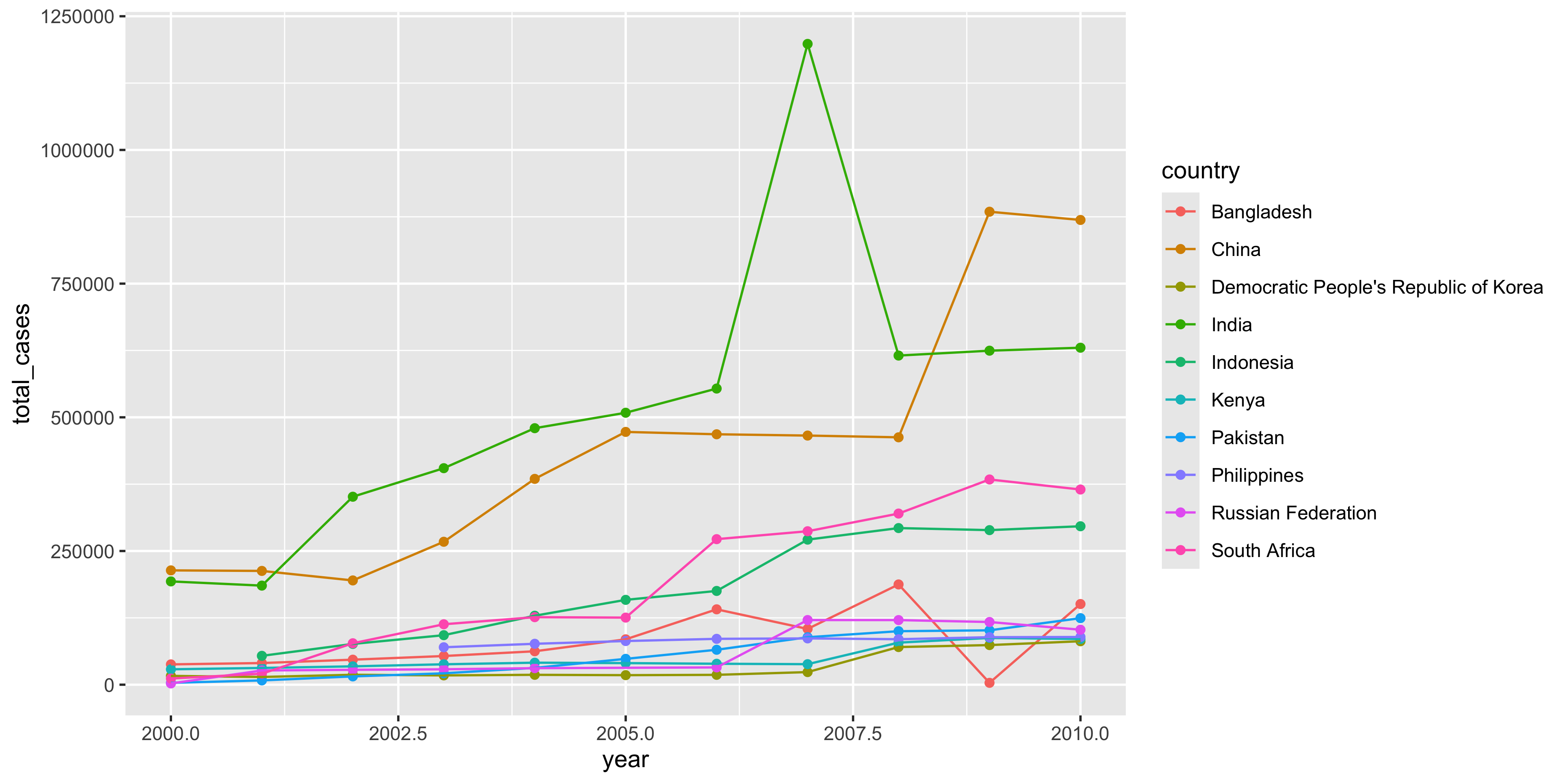
We can extract only the data from the top 10 countries based in 2010 cases and plot how their total case numbers between the years 2000 and 2010.
# A tibble: 10 × 2
   country                               total_cases
   <chr>                                       <dbl>
 1 China                                      869092
 2 India                                      630164
 3 South Africa                               364992
 4 Indonesia                                  296272
 5 Bangladesh                                 150856
 6 Pakistan                                   124455
 7 Russian Federation                         102823
 8 Philippines                                 89198
 9 Kenya                                       85484
10 Democratic People's Republic of Korea       81240
who_tidy %>%filter( country %in% top_10_countries$country, year >=2000, year <=2010 ) %>%summarise(total_cases =sum(cases), .by =c(country, year) ) %>%ggplot(aes(x = year, y = total_cases, col = country)) +geom_point() +geom_line()
5.8 Summary
Today we learned about the concept of “tidy data”. A particular form of tabular data that is particularly suitable for the tidyverse. It contains:
one variable per column
one observation per row
one value per cell
We learned to reshape data frames using various functions powerful functions.
pivot_wider() reduces the number of rows and move information into new columns.
pivot_longer() reduces the number of columns and increase the number of rows. Moving the column names into a new column.
separate() separates multiple values encoded in a single column into individual columns based on a separator character.
We learned to combine data frames using the left_join() function. This allows us to merge data frames together that have common columns, matching up the rows according to the shared column.
left_join(left, right, by = shared_column) takes two data frames and merges them based on the shared_column column. The information from the right data frame is added to the left if there is a match within the shared column.
left_join(left, right, by = join_by(left_col_name == right_col_name)) can be used to join using columns from two data frames that encode the same values but have different column names
We also learned some useful string manipulation functions that help us clean up data columns
str_replace() lets us replace patterns in a string
str_remove() lets us remove patterns in a string
Together these make up a very versatile toolkit for transforming messy data you find in the wild into a tidy, more useful format to summarise information or produce plots with.
Source Code
---filters: - naquizformat: html: toc: true toc-location: left toc-title: "In this chapter:"---# Putting it all together {#sec-chapter05}In this chapter we will combine all the skills we have learned so far to perform a complete analysis of a small dataset.::: {.callout-tip title="Learning Objectives"}At the end of this chapter, learners should be able to:1. Describe the key steps in data analysis (exploration, manipulating and plotting)2. Understand how pivot and join functions can be used to reshape and combine entire data frames:::## Introduction to the datasetIn this chapter we will use the mousezempic dosage data `m_dose` and mouse expression data `m_exp` data frames, which contain information about the mice including mousezempic dose, and their gene expression levels, respectively.```{r}#| eval: false#| include: falsedir.create("data") # create data directory if it doesn't existdownload.file("https://raw.githubusercontent.com/kzeglinski/new_wehi_r_course/refs/heads/main/data/m_exp.tsv", "data/m_exp.tsv") # download data``````{r}#| message: falselibrary(tidyverse)library(patchwork)# read in dosage datam_dose <-read_csv("data/mousezempic_dosage_data.csv")m_dose``````{r}#| message: false# read in expression datam_exp <-read_tsv("data/mousezempic_expression_data.tsv")m_exp```::: callout-noteWe have used `read_csv()` for the mouse data and `read_tsv()` for the expression data.These are for reading data separated by commas and tab characters respectively.The `readr` package also provides `read_delim()` to let the package guess your delimiter, but if you know the format of your file then it's good practice to use the appropriate reading function for more predictable behaviour.:::::: callout-cautionThere's nothing stopping someone from naming a file `file.csv` while having tab-separated data inside.This happens quite often in real-world data so it's a good idea to have a quick look at the data in an text editor before reading it in.:::## Tidy DataThe tidyverse revolves around an important concept called "[tidy data](https://r4ds.hadley.nz/data-tidy.html)".This is a specific representation of tabular data that is considered easy to work with.Tidy data is roughly defined as tabular data that contains:1. Individual variables in columns2. Individual observations in rows3. One data value in each cellHaving individual variables in columns makes then accessible for performing tidyverse operations like `select()`, `mutate()`, `filter()` and `arrange()`.If variables were not stored as columns, then these functions would not be able to access them by name.Having individual observations in rows is important because it associates all variables of each observation with the same row.If the data from one observation is spread across multiple rows then it is easy to incorrect summaries from the `summarise()` function.When using the `filter()` function with tidy data, you can expect to keep all the data for an observation or none at all.When the data for observations is split over different rows, it's possible to unknowingly lose partial data from observations.Having a single value in each cell makes it possible to perform meaningful computations for the values, for example you cannot take a `mean()` of a column of values that contain multiple different values.Although tidy data is the easiest to work with, it's often necessary to alter the format of your data for plotting or table displays.It's a good idea to keep your core data in a tidy format and treating plot or table outputs as representations of that tidy data.::: callout-noteMost data you encounter will not be tidy, the first part of data analysis is usually called "data-wranging" and involves tidying up your data so it is easier to use for downstream analysis.:::## Reshaping and combining data {#sec-reshaping}The `filter()`, `select()`, `mutate()` and `summarise()` functions we learned last chapter all operate along either the columns or the rows of data.Combining these operations cleverly can answer the majority of questions about your data.However, there are two useful families of functions: `pivot` for reshaping your data and `join` for combining your data from shared columns.### Reshaping data with pivot functions {#sec-pivot}Pivoting is a way to change the shape of your tibble.- Pivoting longer reshapes the data to transfer data stored in columns into rows, resulting in more rows and fewer columns.- Pivoting wider is the reverse, moving data from rows into columns.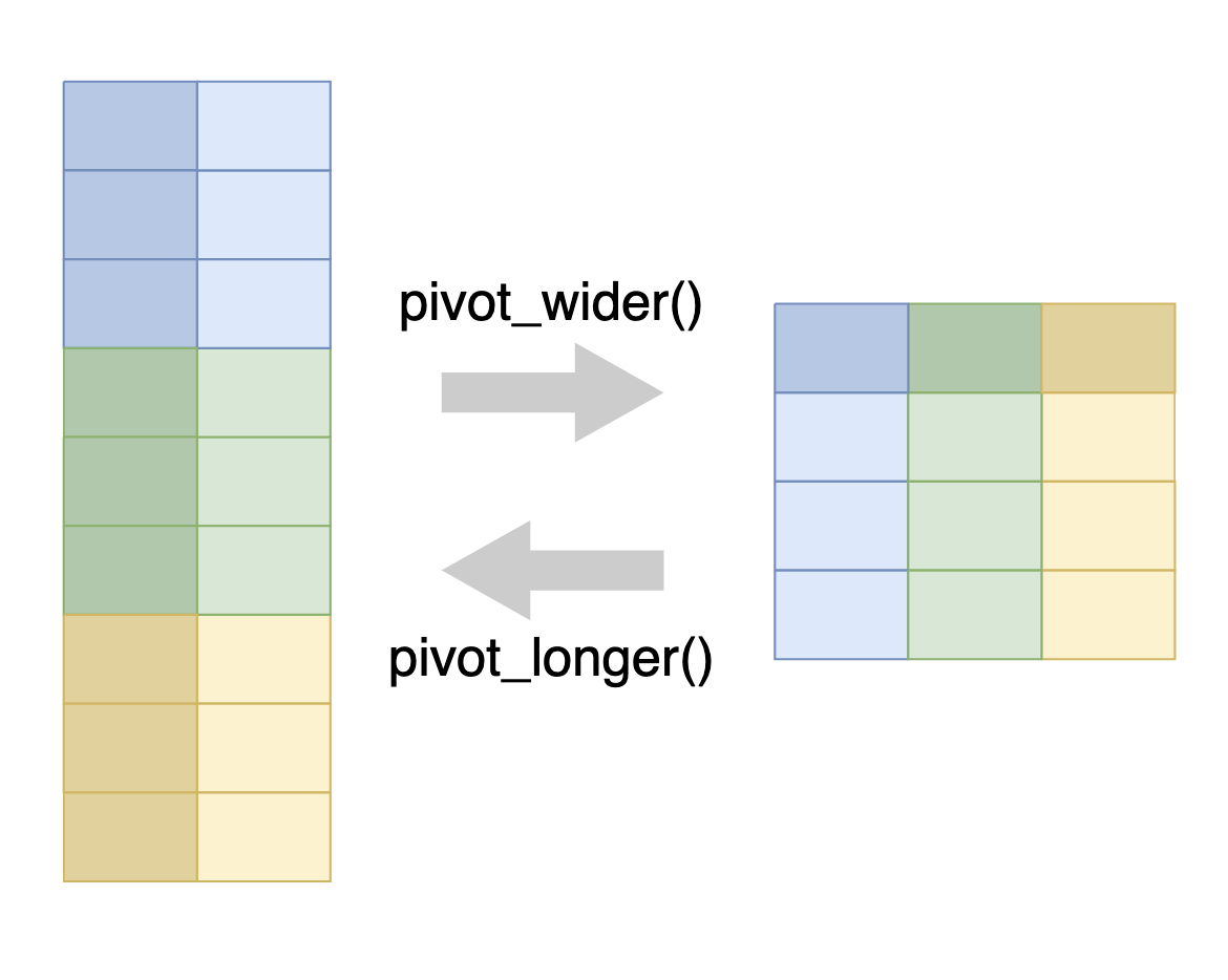{width="50%"}The `pivot_longer()` function is used to pivot data from wide to long format, and the `pivot_wider()` function is used to pivot data from long to wide format.#### Pivot widerA common use case for `pivot_wider()` is to make a [contingency table](https://en.wikipedia.org/wiki/Contingency_table), which shows the number of observations for each combination of two variables.This is often easier to read than the same information in long format.For example, let's say we want to create a table that shows how many mice there are of each strain, in each cage number.We can achieve this in a long format using `summarise()` as we learned in the previous section:```{r}m_dose %>%summarise(n_mice =n(),.by =c(cage_number, mouse_strain))```For the specific task of counting, we can achieve the same effect using the `count()` tidyverse function.```{r}m_dose %>%count(cage_number, mouse_strain, name ="n_mice")```This summarises by each combination of `cage_number` and `mouse_strain`, with the `n()` function giving the count of data belonging to that combination.To get a contingency table, we wish to have the information in the `mouse_strain` column displayed along the column names and the values of `n_mice` becoming the values of the cells in the new table.Since the goal is to make the table wider, we use the `pivot_wider()` function.To achieve this, we instruct the `pivot_wider()` function to take names from the `mouse_strain` column and the values from the `n_mice` column.```{r}m_dose %>%count(cage_number, mouse_strain, name ="n_mice") %>%pivot_wider(names_from = mouse_strain, values_from = n_mice)```This has transformed our data into a contingency table, with `NA` where no data corresponding data exists for the specific `cage_number` and `mouse_strain` combination.We can do the same thing to see how many of each mouse strains is in each of our experiment replicates.```{r}m_dose %>%count(replicate, mouse_strain, name ="n_mice") %>%pivot_wider(names_from = mouse_strain, values_from = n_mice)```#### Pivot longerData can often arrive in the form similar to the contingency table we constructed.Although this data is easy to read, it is difficult to operate on using tidyverse functions because the `mouse_strain` data is now stored in the column names and not inside a column we can use as a variable.In order to make this kind of data tidy, we use the `pivot_longer()` function, which will create a pair of columns from the column names and the value of the corresponding cell.To demonstrate `pivot_longer()`, we will use the `m_exp` that we downloaded earlier.This data frame contains the expression levels of two genes (TH and PRLH) suspected to be upregulated in mice taking MouseZempic, as well as one housekeeping gene (HPRT1), all measured in triplicate.```{r}m_exp```The data is currently in wide format, with each row representing a different mouse (identified by its `id_num`) and each column representing a different measurement of a gene.To reshape this data into a long format (where each measurement is contained on a separate row), we can use `pivot_longer()`, specifying three arguments:1. `cols`: the columns to pivot from. You can use selection helpers like `contains()` or `starts_with()` to easily select multiple columns at once.2. `names_to`: the name of a new column that will contain the original column names.3. `values_to`: the name of a new column that will contain the values from the original columns.In this particular case here's what the code would look like:```{r}m_exp_long <- m_exp %>%pivot_longer(cols =contains("_rep"),names_to ="measurement",values_to ="expression_level" )m_exp_long```::: {.callout-note title="Perplexed by pivoting?"}Pivoting can be a bit tricky to get your head around!Often when you're doing analysis, you'll run into the problem of knowing that you need to pivot, but not knowing exactly what arguments to use.In these cases, it can be helpful to look at examples online, [like those in the R for Data Science book](https://r4ds.hadley.nz/data-tidy.html#sec-pivoting).:::### Separating data in a columnWhen we look at the `measurement` column we see that it contains two pieces of information.The gene being measured and the replicate number separated by "\_".We can use the `separate()` function to split this data into individual columns so that one column does not contain multiple variables.```{r}m_exp_separate <- m_exp_long %>%separate(measurement, into =c("gene", "replicate"), sep ="_")m_exp_separate```### Summarising valuesNow suppose we wanted to combine the gene expression data across replicates by adding them up, we can use the `summarise()` function to do so.```{r}m_exp_rep_summed <- m_exp_separate %>%summarise(expression_level =sum(expression_level),.by =c(id_num, group, gene) )m_exp_rep_summed```We may also want to get the average expression level of each gene within each experimental group and plot it as a bar chart.```{r}m_exp_rep_summed %>%summarise(expression_level =mean(expression_level),.by =c(group, gene) ) %>%ggplot(aes(x = gene, y = expression_level, fill = group)) +geom_col(position ="dodge")```We see that all 3 genes are slightly higher in the treatment group.### Reshaping for plottingSuppose we wanted to plot the value of two genes against each other.We would need the expression values of genes to be in individual columns.However we have lost this structure after using `pivot_longer()`.We can restore it using `pivot_wider()` after we have summarised the replicates.```{r}m_exp_rep_summed_wide <- m_exp_rep_summed %>%pivot_wider( names_from ="gene", values_from ="expression_level")m_exp_rep_summed_wide```With the replicate aggregated expression levels in individual columns, we can now plot the gene expression values against each other.```{r}m_exp_rep_summed_wide %>%ggplot( aes(x = Th, y = Prlh)) +geom_point()```::: {.callout-note title="Practice exercise"}Make all the pair-wise scatter plots and assemble them together using `patchwork`.There should be plots of:Th vs PrlhTh vs Hprt1Prlh vs Hprt1:::### Combining data with join functions {#sec-join}Data analysis typically involves multiple tables of data.Often there will be tables that are contain related information that must be combined to answer the questions you're interested in.Tables that are related to each other tend to have one or more columns in common, and are referred to as "relational data".Combining relational data in useful ways requires the `join` family of functions.In general joins can accomplish two tasks- Add new variables to an existing table containing additional information.- Filter observations in one table based on whether or not they match observations in another table.- Both of the above at the same time.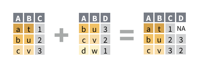A common and basic join is the `left_join()`.It takes two data frame as arguments and optionally a vector of common columns to perform the join on.The reason it's called a left-join because it retains all rows from the left data frame while adding on columns from the right data frame only when the data in the designed joining column(s) match.For example, we can join the `m_dose` data frame with the `m_exp_rep_summed_wide` data frame based on the `id_num` column, which is common to both data frames:```{r}left_join(m_dose, m_exp_rep_summed_wide, by ="id_num")```The `m_dose` contains information about characteristics of each mouse, while the `m_exp_rep_summed_wide` contains the replicate-summed gene expressions of the mice.Each data frame has an `id_num` column that relates the data from the two data frames together, and we have joined them into one table that contains both the data about the mice as well as the expression of their genes.With the `left_join()`, if there is a `id_num` value that exists in the right data frame but not found in the left, then that data will not be present in the joined table.For any `id_num` that appears only in the left but not the right data frame, the values in the newly created columns will be `NA`.::: callout-cautionIf the values from the left data frame matches to multiple rows of the column in the right data frame, the `left_join()` will duplicate the data from the left data frame for each match to the right.This can cause issues with downstream summarisation if not carefully considered.:::#### Joining with mismatched column namesOften the column containing the matching information has different names in different data frames.For example what might be called "id_num" in one data frame could also be called "mouse_id" in another data frame.In those cases the `by` argument of `left_join()` can be formatted to let the function know which column in the left data frame matches to which column on the right.We will demonstrate this by renaming the `id_num` column in the `m_dose` to `mouse_id` and using it to perform the join instead.We will use the `join_by(mouse_id == id_num)` helper function for the `by` argument to specify the different columns we wish to join by.```{r}# rename id_num to mouse_idm_dose_data_new <- m_dose %>%rename(mouse_id = id_num)m_dose_data_new``````{r}# perform left join by matching mouse_id of the left data frame to id_num of the right data framem_joined_data <-left_join( m_dose_data_new, m_exp_rep_summed_wide,by =join_by(mouse_id == id_num)) %>%drop_na() # keep only rows without NAm_joined_data```::: callout-noteWhen joining data frames with mismatched column names, the column name from the left data frame argument will be retained for the joined result.:::::: callout-noteAn older syntax exists for the `by` argument that would look like `by = c("mouse_id" = "id_num")`.This does the same thing as what is shown above but the documentation now recommends the new syntax which allows for flexible options like joining to the closest.:::## Visualising & testing expression between strainsWith the joined data we now have more information about the mice in addition to the expression data.So we can check if there is any significant difference in gene expressions between mouse strains.```{r}m_joined_data %>%ggplot( aes(x = mouse_strain, y = Th, fill = mouse_strain)) +geom_violin()```If we wanted to plot all 3 genes, one way is to make 3 different plots, but we can also use facets.However to use facets we would need to have the faceting variable in a column, and currently our gene names are in the column names.So we must use `pivot_longer()`.```{r}m_joined_data_long <- m_joined_data %>%pivot_longer(cols =c(Th, Prlh, Hprt1), names_to ="gene", values_to ="expression")m_joined_data_long```Now that the gene variable is in a column, we can use this information to create our faceted plot.We use `facet_wrap()` with the `scales = "free_y"` argument so each gene can have its own y-axis.```{r}m_joined_data_long %>%ggplot( aes(x = mouse_strain, y = expression, fill = mouse_strain)) +geom_violin() +facet_wrap(~gene, scales ="free_y")```There doesn't appear to be clear differences in the expression of these three genes between the haplotypes.### Simple linear model (discrete x)To fit a line through the gene expression values of each mouse genotype, and test for significance of the x\~y relationship, we can use a handy function [`lm_test()`](https://github.com/bansell/tidyrstats?tab=readme-ov-file#lm_test) from the `tidyrstats` library.```{r}library(tidyrstats)```This function takes a long-format data frame as input, and the formula for the linear model we want to fit.(We will read more about linear models in later chapters).For this test, for each gene, we want to know whether the response (gene expression ; aka 'y'), changes significantly with the predictor (mouse strain ; aka 'x').The model formula will be `y ~ x1`, that is `expression ~ mouse_strain`.```{r}m_joined_data_long %>%group_by(gene) %>%lm_test(expression ~ mouse_strain) %>%filter(term!='intercept') %>%arrange(gene,term)```Our intuition from the violin plots is correct.None of the genes show significant differences in expression between the Black6 vs the reference (BALBC), nor the CD-1 vs the reference.Note that all of the P values are \> 0.05, meaning we dont have enough evidence to reject the null hypothesis.## Visualising & testing relationships between dosage and genesWith the joined data frame we can also visualise the relationship between the drug dosage and the genes, separated by mouse strain.We do this by using our `m_joined_data_long` to plot with `facet_grid()` specifying the layout of our grid.```{r}m_joined_data_long %>%ggplot(aes(x = drug_dose_g, y = expression, color = mouse_strain)) +geom_point() +geom_smooth(method ="lm") +facet_grid(cols =vars(mouse_strain), rows =vars(gene), scales ="free")```Although very minor, there appears to be some effect of dosage on gene expression that is strain specific.### Simple linear model (continuous x)Again, we can test this using `lm_test()`, where y is `expression`, and x is now the continuous variable `drug_dose_g`.We are testing the association for each gene in each mouse strain, by grouping the input data before `lm_test()`.Note this is different from correcting for gene and mouse strain as covariates, because the model only tests one gene-strain combination at a time.```{r}m_joined_data_long %>%group_by(mouse_strain, gene) %>%lm_test(expression ~ drug_dose_g) %>%filter(term!='intercept') %>%arrange(mouse_strain, gene, p.value)```Here we can see, in fact there is a significant association between Mousezempic drug dose and gene expression: within the Black 6 strain, for the Hprt1 gene.::: {.callout-note title="Stating statistical findings"}From our summary table above, can you finish this sentence which is the formal statement of results from a linear model?*"In the Black 6 mouse strain, for every 1 gram increase in drug dose, on average, Hprt1 gene expression ..."*:::You can read and work through more `lm_test()` examples in the [Statistics in R Primer](stats_primer.qmd).## Saving multiple objectsWe can save our newly transformed and joined data frames for easy access using the `save()` command, which takes any number of environment objects, and a new `Rdata` format file name as arguments:```{r}save( m_exp_rep_summed, m_exp_rep_summed_wide, m_joined_data_long,file ='data_processed/mousezempic_cleaned_joined.Rdata')```## Another case study - WHO tuberculosis dataWe can look at another dataset containing tuberculosis (TB) cases broken down by year, country, age, gender, and diagnosis method.The data comes from the [2014 World Health Organization Global Tuberculosis Report](https://www.who.int/teams/global-tuberculosis-programme/data) and is typical of many real-life datasets in terms of structure.There are redundant columns, odd variable codes and missing values.We want to tidy it up using the tools we have learned in order to try to extract some information from this data.```{r}who```The first thing we notice is that `country`, `iso2` and `iso3` all seem to be different encodings for the country.The `year` column is fine as a variable but the rest of the columns seem appear to be coding values in the column names.There are numeric values in the cells, and since we know this dataset is supposed to contain case numbers, and no column clearly denotes this, we suspect that the values in the columns are case numbers with the column names being descriptive of the cases.Since we believe that many of these column names are in fact encoding data, we want to `pivot_longer()` to put that information in a column for further processing.```{r}# pivot longer with columns 5 to 60, drop NA valueswho_long <- who %>%pivot_longer(cols =5:60, # alternatively contains("_")names_to ="description",values_to ="cases",values_drop_na =TRUE )who_long```It doesn't look like the values in `description` are unique, so we can try to count them to get a sense of what we're dealing with.It will show us the unique values as well as the counts for each value.```{r}who_long %>%count(description)```Some patterns emerge, and it maybe be possible to guess at exactly what these values mean.For example we see the presence of "m" and "f" in the encoding which probably encodes sex.Luckily we have a data dictionary ready from the source that tells us what this means.1. The first part tells us if the data is new or old, in this case all data is new.2. The next part describe the type of TB:- `rel` for relapse- `ep` for extrapulmonary- `sn` for pulmonary TB that cannot be diagnosed with a pulmonary smear (smear negative)- `sp` for pulmonary TB that can be diagnosed with a smear (smear positive)3. The sex of the patient. Males and females denoted by `m` and `f` respectively.4. The 7 age groups the data is divided into:- `014`: 0 - 14 years old- `1524`: 15 - 24 years old- `2534`: 25 - 34 years old- `3544`: 35 - 44 years old- `4554`: 45 - 54 years old- `5564`: 55 - 64 years old- `65`: 65 or older### String manupulationArmed with that knowledge we can begin to tidy up our dataset!The first thing we will do is tidy up the `description` column, we will do this with some string manipulation functions from the tidyverse.These functions help us manipulate strings programatically and are essential in dealing with real-world data.Some useful functions for string manipulation include:- `str_replace(string, pattern, replacement)`: replaces the pattern in the string with the replacement.- `str_extract(string, pattern)`: extracts the part of the string matching the pattern.- `str_remove(string, pattern)`: removes the part of the string matching the pattern.The full list of functions can be found in the [stringr package documentation](https://stringr.tidyverse.org/reference/index.html) and patterns can be written in very powerful ways with [regular expressions](https://r4ds.had.co.nz/strings.html#matching-patterns-with-regular-expressions).For our purposes we will just use simply fixed patterns.We saw previously that we can use `separate()` to break apart on column into multiple columns.However, we see there is a problem in this dataset where the cases that are marked as relapse are encoded `newrel` which doesn't leave us with a separator to use.We can remedy this by using a combination of `mutate()` and `str_replace()` to replace all instances of `newrel` with `new_rel`.```{r}who_long <- who_long %>%mutate(description =str_replace(description, "newrel", "new_rel"))who_long```Since every single observation contains only new cases and no old cases, the `new_` portion of the encoding is redundant.So we can remove it using `str_remove()`.```{r}who_long <- who_long %>%mutate(description =str_remove(description, "new_"))who_long```Now one last problem remains, there is no separator between the sex and age group.So we can once again use `str_replace()` to edit in an underscore.Note that we use `"_f"` and `"_m"` as our patterns as a precaution in case the letters naturally occur elsewhere in the encoding.```{r}who_long <- who_long %>%mutate(description =str_replace(description, "_f", "_f_")) %>%mutate(description =str_replace(description, "_m", "_m_"))who_long```With that we are finally able to separate the data into individual columns with `separate()`.```{r}who_separated <- who_long %>%separate(description, into =c("type", "sex", "age_group"), sep ="_")who_separated```Because the columns `iso2` and `iso3` contain redundant information about the country, we can remove them, but also retain them for reference as we may want to know what the short forms of the countries are when relating it other tables.To do so we can `select()` the columns containing this information, then use `distinct()` to keep only unique rows.```{r}country_codes <- who_separated %>%select(country, iso2, iso3) %>%distinct()country_codes```With that we can safely remove the redundant information from our data and end up with a tidy data frame.```{r}who_tidy <- who_separated %>%select(-iso2, -iso3)who_tidy```From there we can easily visualise various aspects of the data for analysis.For example we can see what country had the highest number of total cases in the year 2010.```{r}who_tidy %>%filter(year ==2010) %>%summarise(total_cases =sum(cases), .by = country) %>%arrange(desc(total_cases))```We can extract only the data from the top 10 countries based in 2010 cases and plot how their total case numbers between the years 2000 and 2010.```{r}top_10_countries <- who_tidy %>%filter(year ==2010) %>%summarise(total_cases =sum(cases), .by = country) %>%arrange(desc(total_cases)) %>%slice(1:10)top_10_countries``````{r}who_tidy %>%filter( country %in% top_10_countries$country, year >=2000, year <=2010 ) %>%summarise(total_cases =sum(cases), .by =c(country, year) ) %>%ggplot(aes(x = year, y = total_cases, col = country)) +geom_point() +geom_line()```## SummaryToday we learned about the concept of "tidy data".A particular form of tabular data that is particularly suitable for the tidyverse.It contains:- one variable per column- one observation per row- one value per cellWe learned to reshape data frames using various functions powerful functions.- `pivot_wider()` reduces the number of rows and move information into new columns.- `pivot_longer()` reduces the number of columns and increase the number of rows. Moving the column names into a new column.- `separate()` separates multiple values encoded in a single column into individual columns based on a separator character.We learned to combine data frames using the `left_join()` function.This allows us to merge data frames together that have common columns, matching up the rows according to the shared column.- `left_join(left, right, by = shared_column)` takes two data frames and merges them based on the `shared_column` column. The information from the right data frame is added to the left if there is a match within the shared column.- `left_join(left, right, by = join_by(left_col_name == right_col_name))` can be used to join using columns from two data frames that encode the same values but have different column namesWe also learned some useful string manipulation functions that help us clean up data columns- `str_replace()` lets us replace patterns in a string- `str_remove()` lets us remove patterns in a stringTogether these make up a very versatile toolkit for transforming messy data you find in the wild into a tidy, more useful format to summarise information or produce plots with.<!-- :::::::::::::::::::: {.callout-important title="Practice exercises"} --><!-- Try these practice questions to test your understanding --><!-- :::::::: question --><!-- 1\. What does the following code do? --><!-- ```{r} --><!-- #| eval: false --><!-- m_dose %>% --><!-- summarise( --><!-- med_tail = median(tail_length_mm, na.rm = TRUE), --><!-- .by = c(mouse_strain, sex)) %>% --><!-- pivot_wider(names_from = sex, values_from = med_tail) --><!-- ``` --><!-- ::::::: choices --><!-- ::: choice --><!-- Pivots data into a wide format where there is a column for each sex. --><!-- ::: --><!-- ::: {.choice .correct-choice} --><!-- Calculates the median tail length for each unique combination of `mouse_strain` and `sex` in the `m_dose` data frame, then pivots into a wide format where there is a column for each sex. --><!-- ::: --><!-- ::: choice --><!-- Calculates the median tail length for each unique combination of `mouse_strain` and `sex` in the `m_dose` data frame, then pivots into a wide format where there is a column for each mouse strain. --><!-- ::: --><!-- ::: choice --><!-- It just gives an error --><!-- ::: --><!-- ::::::: --><!-- :::::::: --><!-- 2\. I have run the following code to create a new column in the `m_dose` data frame that gives the weight of the mice at the end of the experiment. --><!-- ```{r} --><!-- m_dose %>% --><!-- # add a column for the weight at the end of the experiment --><!-- mutate(final_weight_g = initial_weight_g - weight_lost_g) %>% --><!-- # select the relevant columns only --><!-- select(id_num, initial_weight_g, final_weight_g) --><!-- ``` --><!-- Which pivot function call would I use to take this data from a wide format (where there is a column for the final and initial weight) to a long format (where there is a row for each mouse and each weight measurement)? --><!-- ::::::: choices --><!-- ::: choice --><!-- `pivot_longer(cols = c(initial_weight_g, final_weight_g), names_to = "weight", values_to = "timepoint")` --><!-- ::: --><!-- ::: choice --><!-- `pivot_longer(cols = c(id_num, final_weight_g), names_to = "timepoint", values_to = "initial_weight_g")` --><!-- ::: --><!-- ::: choice --><!-- `pivot_wider(names_from = initial_weight_g, values_from = final_weight_g)` --><!-- ::: --><!-- ::: {.choice .correct-choice} --><!-- `pivot_longer(cols = c(initial_weight_g, final_weight_g), names_to = "timepoint", values_to = "weight")` --><!-- ::: --><!-- ::::::: --><!-- :::::::: question --><!-- 3\. Which of the following is NOT a valid way to join the `m_dose` data frame with the `m_exp` data frame based on the `id_num` column? --><!-- ::::::: choices --><!-- ::: choice --><!-- `m_dose %>% left_join(m_exp, by = "id_num")` --><!-- ::: --><!-- ::: choice --><!-- `left_join(m_dose, m_exp, by = "id_num")` --><!-- ::: --><!-- ::: {.choice .correct-choice} --><!-- `m_dose %>% left_join(m_exp, .by = "id_num")` --><!-- ::: --><!-- ::: choice --><!-- `m_dose %>% left_join(m_exp, by = ("id_num" = "id_num"))` --><!-- ::: --><!-- ::::::: --><!-- :::::::: --><!-- <details> --><!-- <summary>Solutions</summary> --><!-- 1\. The code first calculates the median tail length for each unique combination of `mouse_strain` and `sex` in the `m_dose` data frame, then pivots the data into a wide format where there is a column for each sex in the dataset (because of the argument `names_from = sex` ) --><!-- 2\. The correct pivot function call to take the data from a wide format to a long format is `pivot_longer(cols = c(initial_weight_g, final_weight_g), names_to = "timepoint", values_to = "weight")`. This code tells R to pivot the `initial_weight_g` and `final_weight_g` columns into a long format, where there is a row for each mouse and each weight measurement. The `names_to` argument specifies to make a column called 'timepoint' that tells us whether the measurement is initial or final, and the `values_to` argument specifies the name of the new column that will contain these measurements. --><!-- 3\. The line of code that is NOT a valid way to join the `m_dose` data frame with the `m_exp` data frame based on the `id_num` column is `m_dose %>% left_join(m_exp, .by = "id_num")`. This line of code is incorrect because the `.by` argument is not used in the `left_join()` function (this can be confusing! it's `.by` when grouping by `by` when joining). The other options are valid ways to join the two data frames based on the `id_num` column: remember that we don't have to use pipes to join data frames, we can use the `left_join()` function directly, and we can use a named vector to specify the columns to join on (although here it's a bit redundant as the columns have the same name). --><!-- </details> --><!-- :::::::::::::::::::: --><!-- summary - Reshaping data with `pivot_longer()` and `pivot_wider()` to change the structure of your data frame. --><!-- - Combining data with `left_join()` to merge two data frames based on a common column. --><!-- questions etc --><!-- 4. Using the `m_dose` data frame, write R code to: --><!-- a. Make a data frame that shows the number of mice of each strain, in each replicate. --><!-- b. Pivot this data frame into a wide format to create a contingency table. --><!-- c. Pivot the wide data frame from (b) back into a long format. --><!-- 5. Let's say I have two data frames, `df1` and `df2`, that I want to join based a shared 'key' column, that is called 'key' in `df1` and 'item_key' in `df2`. Write R code to join these two data frames using the `left_join()` function. --><!-- solutions --><!-- 4. Here's how you could write R code to achieve the tasks: --><!-- a. `m_dose %>% summarise(n_mice = n(), .by = c(mouse_strain, replicate))` --><!-- b. `m_dose %>% summarise(n_mice = n(), .by = c(mouse_strain, replicate)) %>% pivot_wider(names_from = replicate, values_from = n_mice)` --><!-- c. `m_dose %>% summarise(n_mice = n(), .by = c(mouse_strain, replicate)) %>% pivot_wider(names_from = replicate, values_from = n_mice) %>% pivot_longer(cols = starts_with("rep"), names_to = "replicate", values_to = "n_mice")` --><!-- 5. To join the two data frames you could use `df1 %>% left_join(df2, by = c("key" = "item_key"))` (with pipe) or `left_join(df1, df2, by = c("key" = "item_key"))` (without pipe). -->